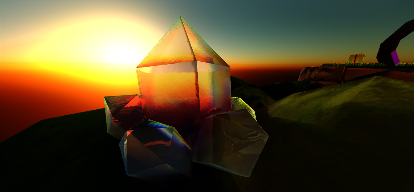
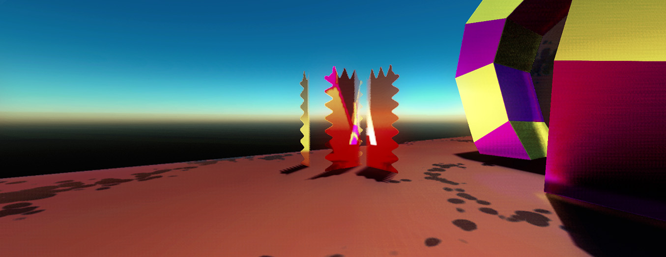
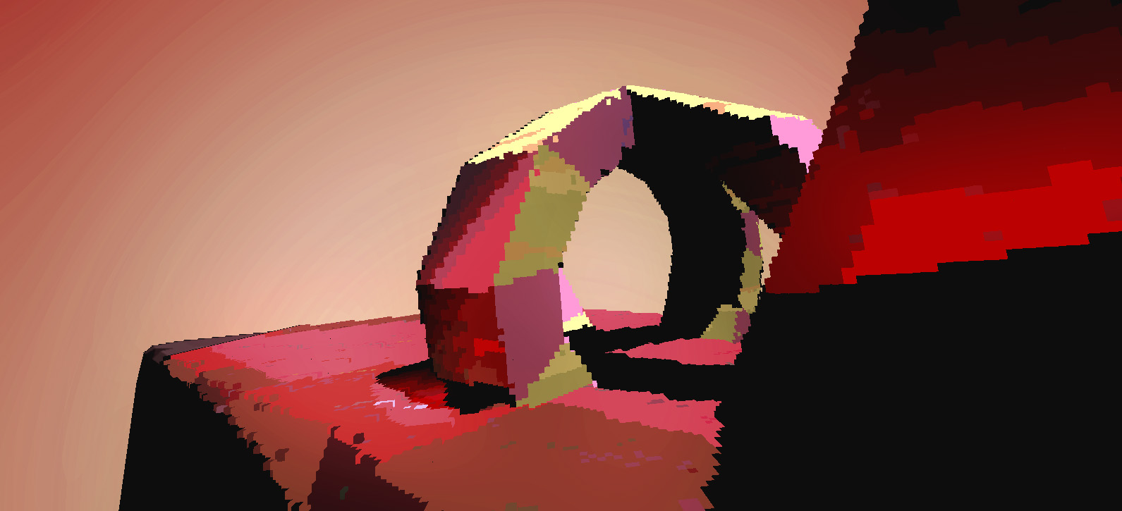
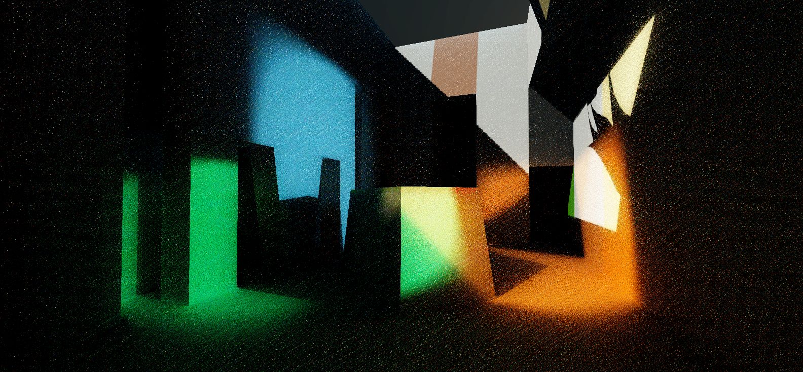
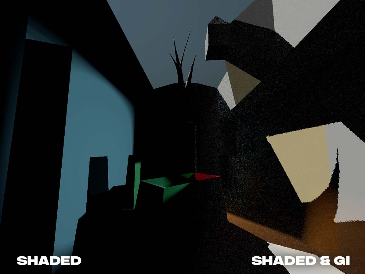
A recently encountered rough glass shader sparked ideas of how to implement not just simple rough translucence, but rather full screen space refraction in a real-time rendering context. This effect is rarely prominently featured, but is able to produce some stunning visuals - especially, when combined with strong light sources & variable surface roughness leading to variably blurry translucence.
To get such refractions working, we require the addition of mesh categories, in order to selectively re-render parts of the scene (the transparent meshes). Those categories are associated with the render object LOD data, hence can be accessed by the occlusion-culling setup to selectively push corresponding instance draw calls into a separate buffer (offset).
Now, rather than simply rendering transparent geometry to the G-Buffer, like all the other objects (which would make it impossible to apply deferred shading to the occluded objects) - and writing to the same depth buffer as those would pollute our occlusion culling HZB with transparent meshes, which would reveal the culling procedure - we draw this transparent geometry to a separate transparency-g-buffer (Color, Transparency, Normal, Roughness, IOR + separate depth) using backface-culling and then we draw those meshes once more to a depth-only framebuffer using frontface-culling. This leaves us with the entry & exit depth of the transparent surfaces at every pixel, as well as the corresponding deferred shading information.
Now, after we've rendered all of our usual suspects, we apply regular deferred shading & GI to them. The resulting texture is then blit to a lower resolution & quality texture, and blurred mips are computed.
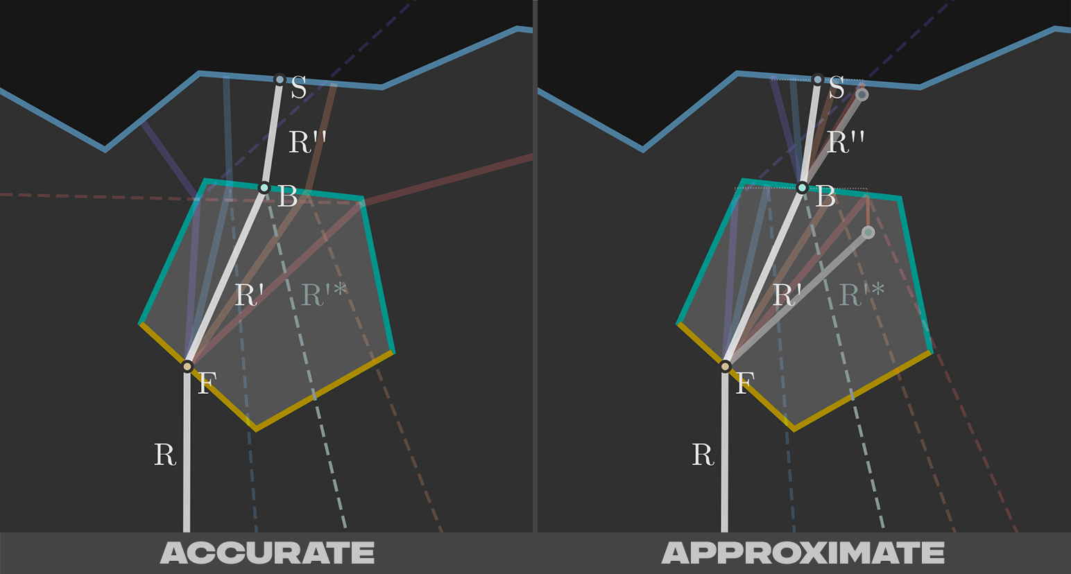
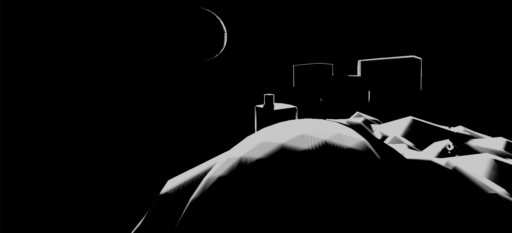
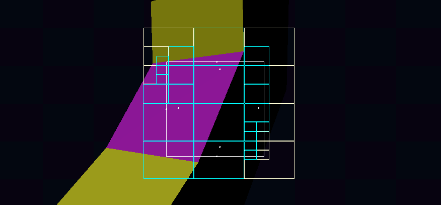
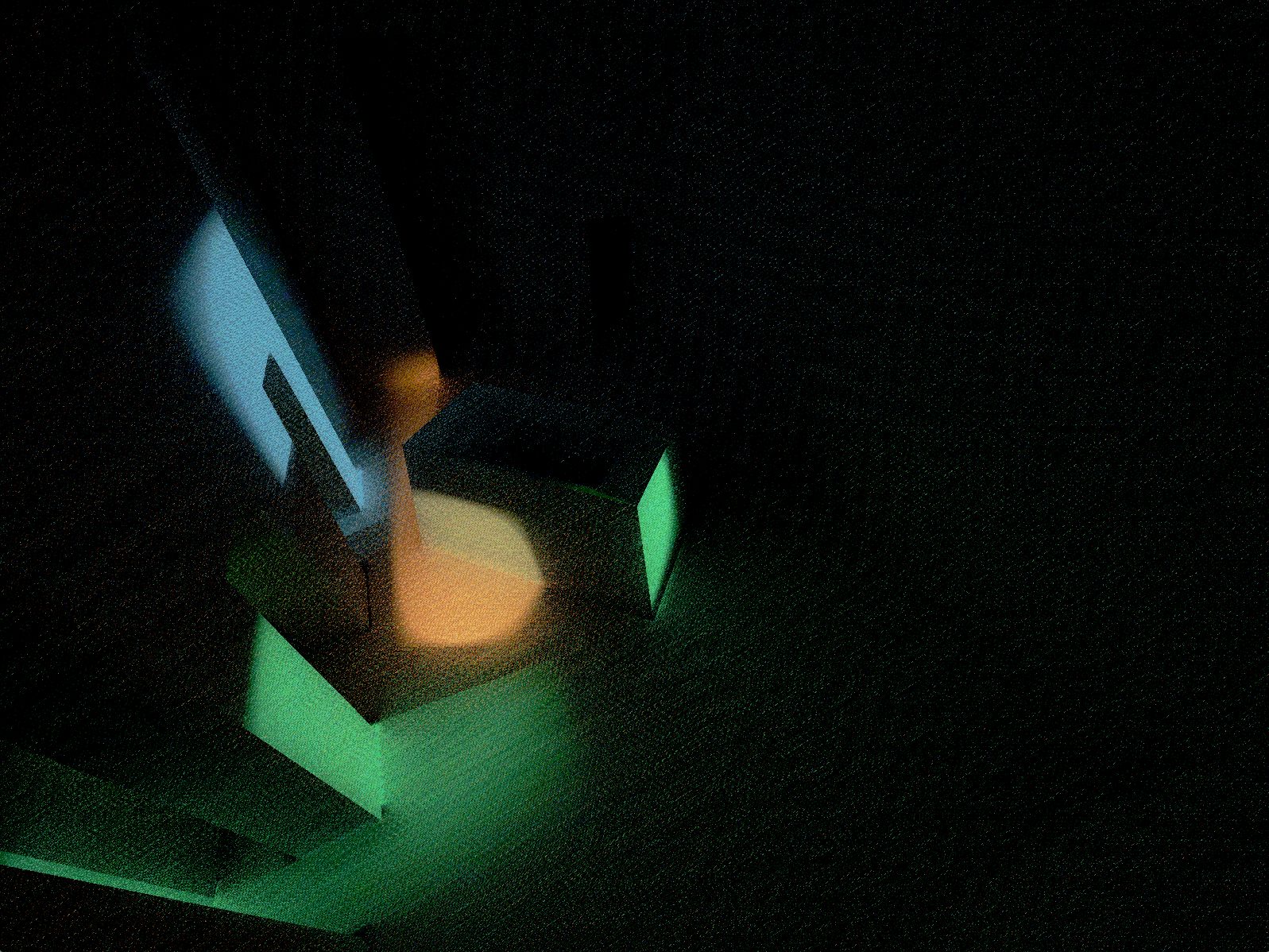
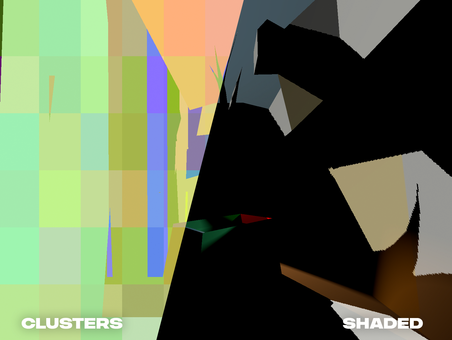
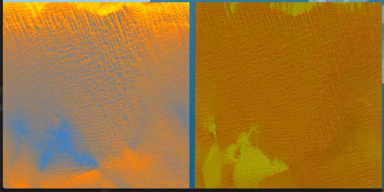
This leaves us with the following slice through the rendered scene geometry (when observed from above, so the further up, the futher away a pixel is from the camera, left to right is a flattened view of what's actually on screen)
Yellow: Transparent Front-Face Depth Turquoise: Transparent Back-Face Depth Dark Blue: Scene Depth
Tracing Refractions
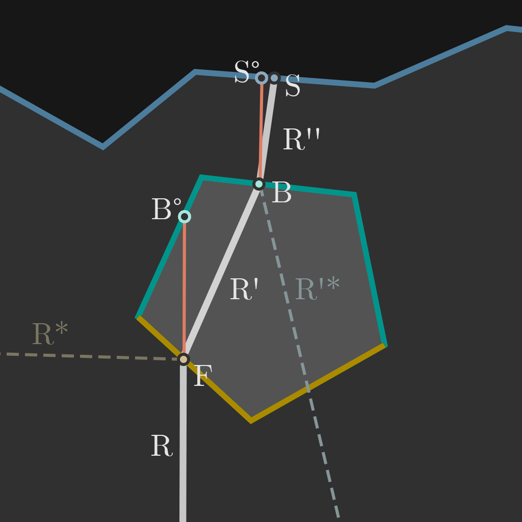
Having the information about the depth of the back- & front-face doesn't give us a complete picture of the encompassed geometry (essential parts of the mesh may be covered by a stray backface & we only have knowledge about the information that's actually on-screen), but it gives us a decent approximation of it, if we simply assume that the entire area between front- & back-face is the only range covered by our transparent object for a given pixel.
With an IOR of 1, we'd even be able to correctly trace though the given geometry - as the rays would simply pass through the mesh unaffected by any refraction angles (so, R would continue towards B°), however, if an IOR != 1 comes into the picture, rather than being able to continue through to B°, we wanna continue via R' to B instead.
To achieve this, we unfortunately can't simply read from a known location, but we'll have to trace our way there. Naively going step-by-step however would be hugely inefficient, so we take the distance FB as a reference point along the direction of R' and use an adaptive Newton-Approach to narrow in on the actual view-space intersection point B on the back-face depth and R'.
      // let's take half the reference-depth as an initial guess

vec3 traceDir = traceStart * (referenceZ / traceStart.z) * 0.5;

for (int it = 0; it < MaxNewtonSteps; it++)

{

  vec3 viewPos = traceStart + traceDir;

  // ...


  if (backFaceDepth < sceneDepth) // if inside transparent obj

  {

    if (nextPos.z < to_screen_depth(viewPos.z))

    {

      // new best hit found!

      traceStart = viewPos;

      // ...

    }

    else // sample hit behind expected ray depth: let's narrow in on previous best guess

      traceDir *= 0.5;

  }

  else // if outside: let's narrow in on previous best guess

    traceDir *= 0.5;

}
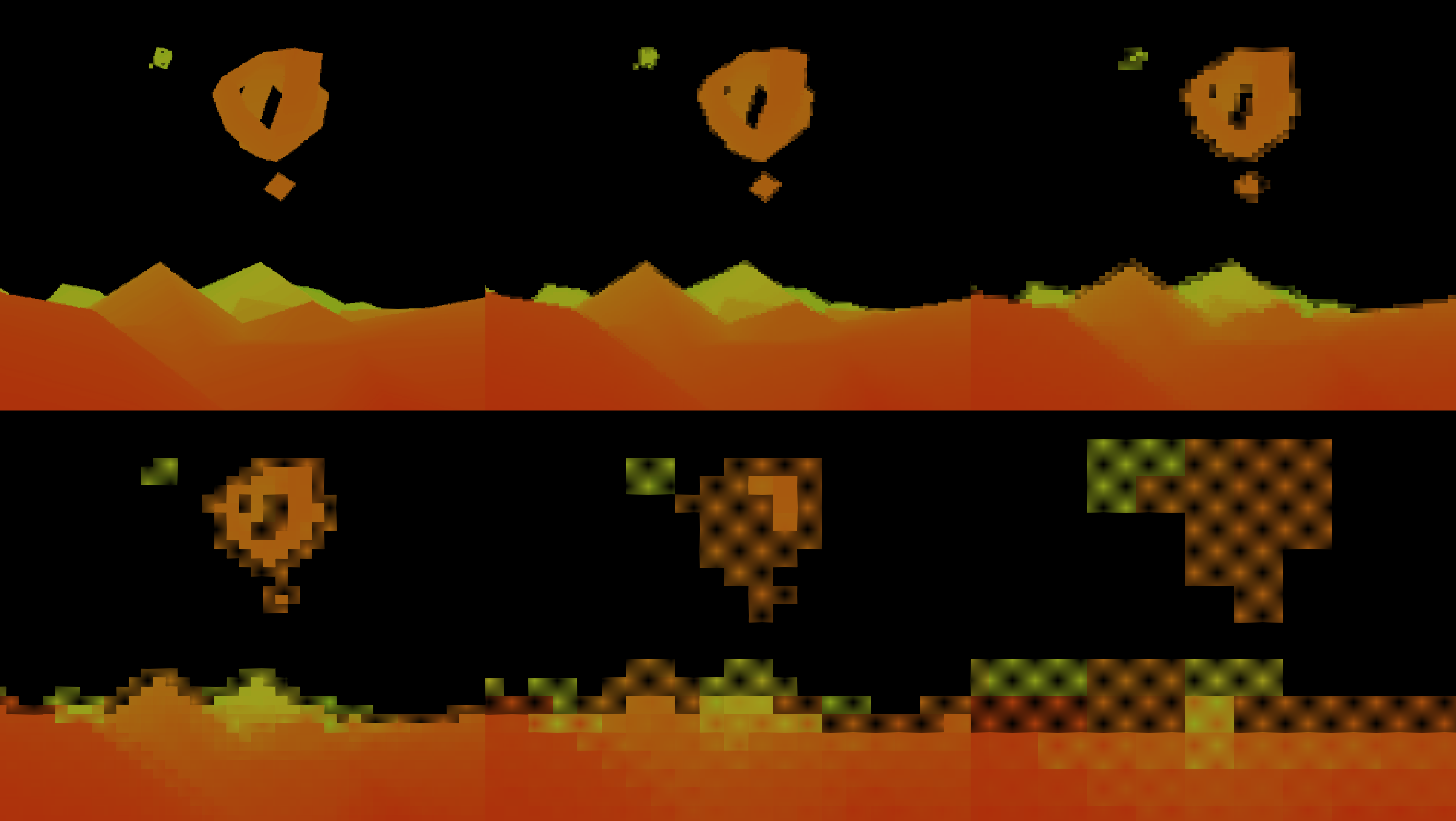
This method is great at finding the approximate area of the intersection, but it'll still result in a jagged appearance even with considerably high values of MaxNewtonSteps:
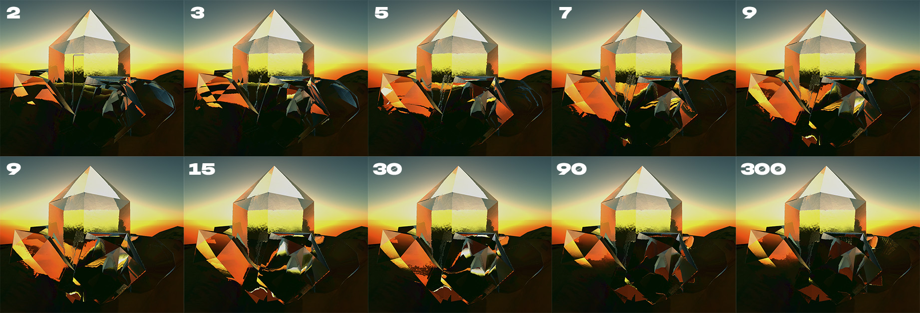
To alleviate - or sometimes even outright resolve this, we can compute the intersection between the screen depth of the last two viewPos and backFaceDepth values (and bound the resulting factor to something like -0.5 ~ 1.5 to restrict the intersection to reasonable values). This produces very good results (especially for flat surfaces) even with fairly low values for MaxNewtonSteps (we chose 9 for a decent balance between performance and accuracy). If we simply sample from the resulting direction of the environment-map (using surface roughness at F to pick a suitable mip layer) with varying number of samples, we get:
Resulting image with N=MaxNewtonSteps
Top Row: Values <= 9
Bottom Row: Values >= 9
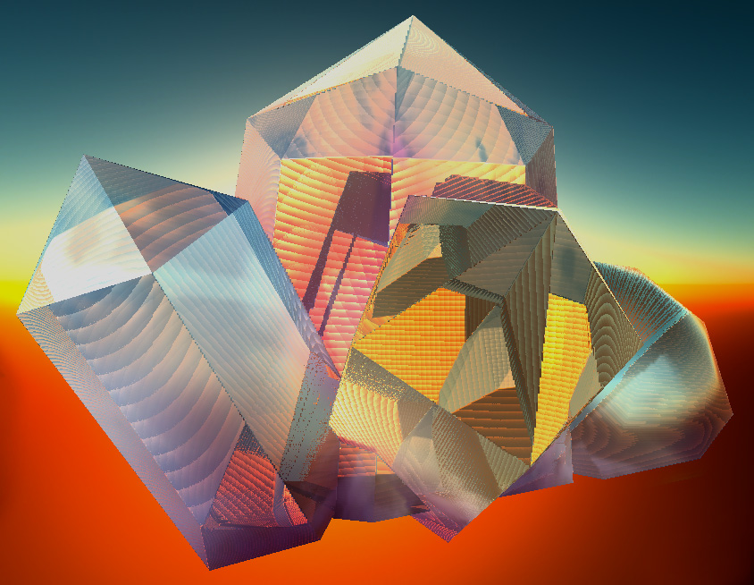
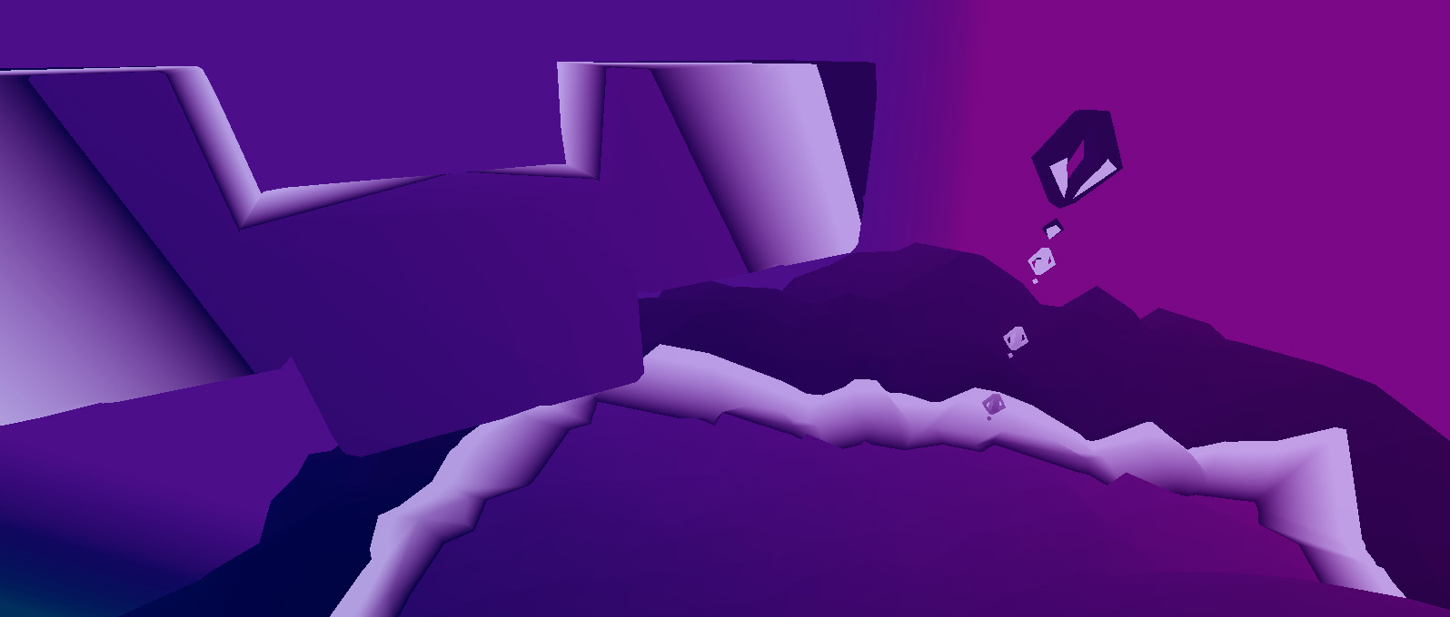
If we compliment this with environment-map samples for first reflection along R* (interpolating via Schlick's approximation for the Fresnel reflectance), this already leads to very impressive looking results. Although, obviously there's not just external reflections to deal with, but also internal reflections. There are technically infinitely many of them, but again, the most significant contribution can be somewhat easily approximated from the first internal reflection along R'* by reflecting R along the normal at B.
Unfortunately, we don't have the normal at the backface though - we only wrote the depth, so we'll have to resurrect the approximate normal by reading two samples in screen space from the neighboring pixels of our back-face depth, as we're able to simply calculate a normal from the differences. Same reading from environment-map in the direction of R'*and interpolating the result with the refracted color via Schlick's approximation as before and we're one step closer to the final result.
This works well with higher IOR, but for IOR = 1, the missing scene geometry from the environment-map is very apparent. So, let's use a slightly altered version of the screen-space tracing method from above to complete the journey and trace along R'' for S, taking the distance BS° as our reference length. The most annoying case to handle here is, that for certain pixels, the resulting depth reaches the far-plane, which may not lend itself well to the final interpolation stage. Just like before, we take the surface roughness at F to read from the correspondingly blurred version of the shaded scene (or environment-map, if the depth reaches the far-plane).
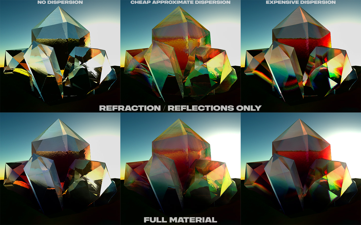
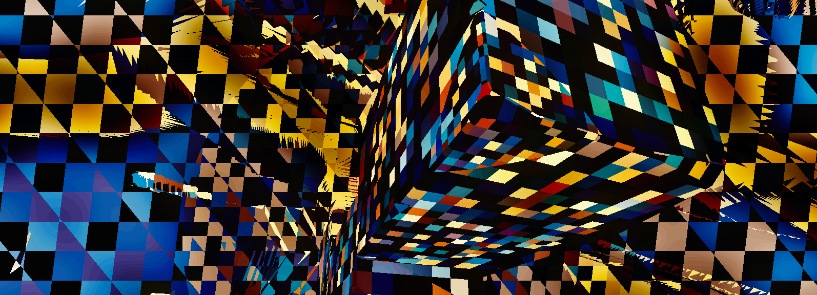
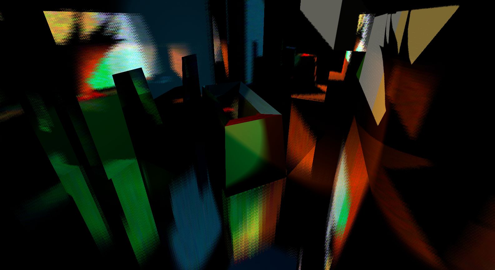
All the colors of Dispersion
Dispersion is the property which describes the way a prism splits white light into all the colors of the rainbow. To add dispersion into the picture, we may simply sum up our material samples from above with only our IOR varying slightly, by taking a value k slightly larger than 1 and iteratively stepping over n samples of the material with IOR between IOR * 1 / k ~ IOR * k.
To get those samples to be colored like the rainbow, we calculate a bunch of RGB color values that correspond to the visible wavelengths of light (approximately 380 nm ~ 780 nm) using a tool like this. As the "rainbow" will overlap with itself, the colors in the center will not appear as saturated, so we'll correct for that - and lastly we divide the resulting color by the overall tint, to have "white" transparent surfaces actually appear untinted. As these colors don't change during runtime, we may simply precalculate them into a lookup-table.
Now, simply summing up the traced (and re-traced) scene for those N IORs (for which we'd each apply the pre-calculated tint) is obviously very expensive - but it'll generate quite an accurate & nice looking result.
The far more inaccurate, but significantly cheaper version is to extrapolate some of the values along the way: So, after we've found B, we take R' and calculate how far the direction of our boundary IOR values would shift the position of the corresponding points B for this IOR (assuming the same distance traveled through the transparent medium) on screen. This is obviously quite far from the real scenario, but it's at least a close guess.
Now, our goal is to eventually sum up all the blended refractions & inner reflections and tint them in the color that corresponds to the deviated IOR value. Let's first focus on the inner reflections: If we assume that the on-screen span of the IOR-range will be linear, we can simply read from (N-1)/2 positions between the center and each boundary, calculate the normal there (just like we did for the non-dispersed version, by simply checking the neighboring depth values and resurrecting an approximated normal that way), calculate the reflected direction with this normal and the direction resulting from initial refraction using the corresponding IOR.
This leaves us with the refracted part: Unfortunately tracing from the much more accurate dispersed position B on the backface-depth would require expensive re-tracing, but we'd much rather just do something that's akin to our first-refraction. So, to mirror that, by refracting the dispersed R' again with the IOR corresponding to the current sample with the previously calculated normal at the dispersed position B to get a dispersed R'', but placed at the non-dispersed point B and extend it to the same length that the non-dispersed R'' had, leaving us with an approximated dispersed S. If we translate that position to screen coordinates and read from either the shaded scene or the environment-map (depending on if the depth there is at the far-plane) - again choosing the mip-level that corresponds to the surface roughness at F -, we now have a rough guess of what our dispersed color at S should be.
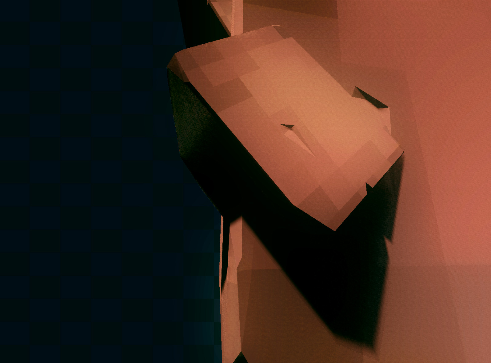
To finalize the look, we blend between the assumed dispersed inner-reflection R'* and the assumed dispersed refraction R'' via Schlick's approximation for the Fresnel reflectance and tint the result with the (partially desaturated) wavelength equivalent color from our lookup-table. Et voilà: Certainly not perfect, but it has the visual appearance of a transparent material with proper dispersion. Interestingly, one of the more important visual aspect of dispersion appears to be the slight blurring of the background, which provides clear visual feedback about whether we're seeing the front or the inside of the transparent object.
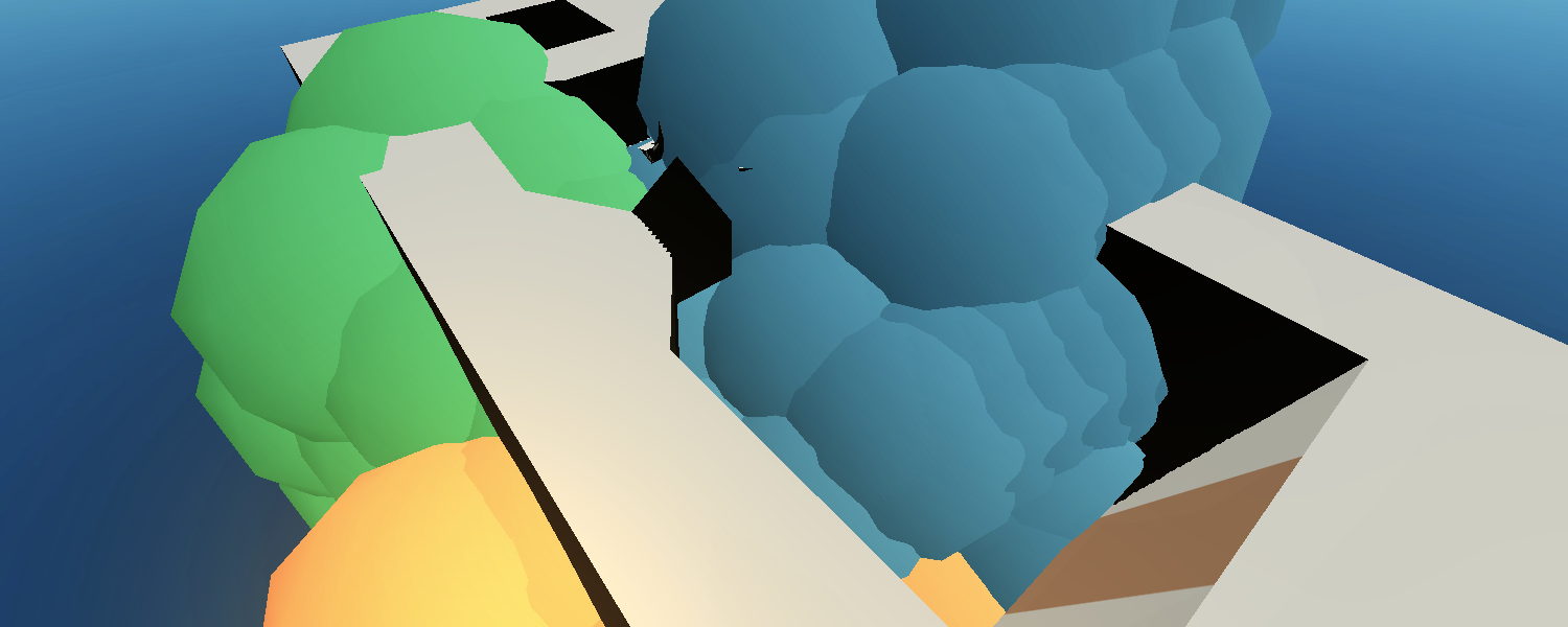
Assembling Seamless Meshes
In order to provide a huge variety of trees without requiring each and every tree to be a separate mesh (requiring a huge amount of resources), our preferred approach is - rather than having pre-prepared meshes of full trees - assemble them out of reusable segments which can be combined in a vast number of different ways achieving a huge space of possibilities even within comparatively restrictive memory requirements.
As it's unreasonable to expect anyone to assemble segments seamlessly via simple placing by hand (not to speak of the horrendous inconvenience) - our first component is an automated "segment-analyzer":
Automated Segment Analysis & Categorization
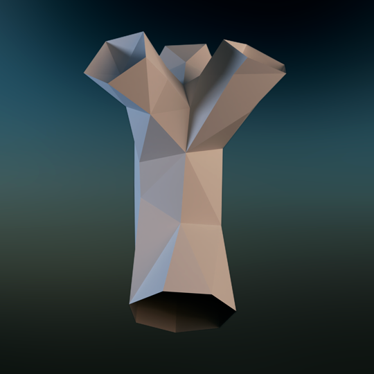
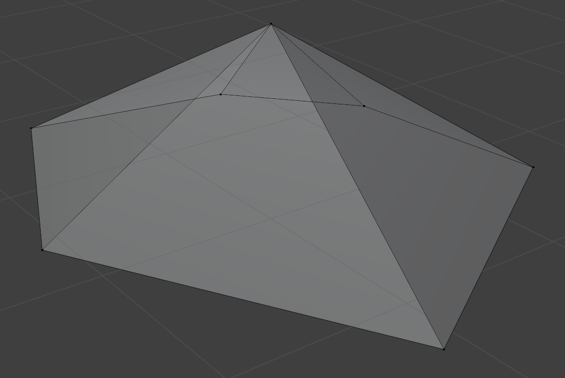
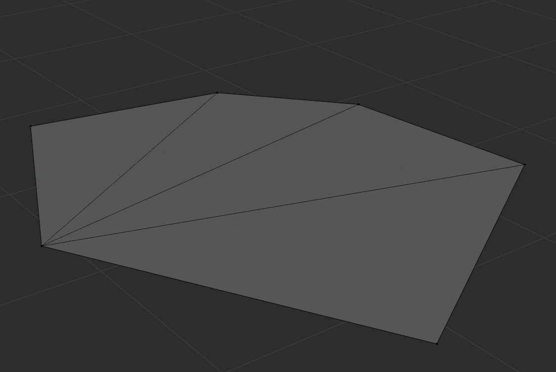
Let's assume, that tree segments are small meshes with multiple openings in the shape of a regular polygon (but with a varying amount of vertices), just like this one:
As should be apparent, this mesh has four openings: One regular heptagon at the bottom and three regular pentagons at the top.
Finding Edges
To get started, let's categorize out vertices in a way where each vert contains a reference to the tris it appears in. We've placed an arbitrary limit of six triangles on this list, as we didn't have any examples where edge-vertices (the only thing relevant for this process), were referenced in more tris than that. In order to identify a point on an opening edge, let's iterate over all triangles it occurs in and note how many times each other vertex is visited by this process. There should be two vertices, which are only visited once - those are the ones that lie on the same edge as the one we started with. If we're unable to find two such neighboring vertices, then move on with the next candidate.
Now, that we've found the edge, we can compute the opening direction (= plane normal), via the cross-product of the vectors to each of the neighboring vertices we selected. As there's always two normalized orthogonal vectors to a plane, let's pick a random point from the triangles we share with any of our selected vertices and compare its direction to the computed opening direction; If it lies in the same hemisphere as our opening direction (= dot product of the direction vs the direction to the shared vertex), we flip our opening direction.
Calculating Openings
Let's take those three points we've selected so far as a starting point and continue further from one end: Again, we iterate over all the triangles this vertex occurs in and mark all vertex occurences - but this time, we ignore all vertices that are already in our current chain (except the first vertex, which we will eventually match to determine that our opening has been completed). Just as before, we pick the one that only appears once - and therefore must lie on an edge; and having found this continuation vertex, we repeat the process until we finally match the first vertex again.
Having calculated the opening direction & corresponding opening plane, we can ensure at every step, that our newly matched vertex actually fits our criteria, and discard it otherwise - potentially even discarding the entire chain in the process.
As we've now found our opening vertices, we average them to determine the center point and take the distance from the first vertex to the center as the radius.
Determining the Rotation Offset
Given a certain center point, radius and plane and number of vertices, there's still infinitely many regular polygons fit this description - we need another factor, a rotation offset from some arbitrary origin, to narrow it down to exactly one unique match, but how can we determine this rotation offset?
There is technically a nice closed-form expression for this conundrum, but unfortunately the inaccuracies appear to explode so quickly, that it isn't of particularly great use to us. What now? - Iteratively narrowing Approximation to the rescue!
Let's first define a transform which should be able to produce our reference point in the plane: (assuming a left-handed coordinate system, with z pointing down)
const quaternion rot = segment_quaternion(up, rotation_offset);
const vec3f point = center + matrix_from_quaternion(rot).transform(vec3f(radius, 0, 0));
Now, with the free parameter rotation_offset, we can gather the diff from our observed location vs the values [0 ~ ]τ to find the appropriate value. Rather than blindly trying to iterate over the given value range, we can sample the difference function at a bunch of fixed positions in this range - let's say every ½π - and then grab the two values surrounding the value with the lowest error (n_min - ½π, n_min + ½π, to account for the spherical implications of those factors) and use Brent's Method to find the minimum in the provided range. As there are vertex_count symemtrical variants of each of those matches, we can even reduce the offset further via the following:
if (rotation_offset > symmetry_angle / 2)
rotation_offset -= symmetry_angle;
Assembling Meshes
Starting with the pre-analyzed segments, we can easily categorize them by the significant opening's number of vertices (we'll pick the largest one - or the one that's closes to [0, 0, 0] as the "significant" or "base"-opening). Now, we start with a randomly picked segment of a chosen category.
To continue, let's first zoom out a bit: Each of the segments is defined in its own segment-space (the direction the significant opening points to, the scale of the opening and its rotation offset). Additionally, there's a local position, rotation & scale at each of the openings of any placed segment in world-space. These two factors have to be considered separately when generating seamless segments. Let's consider those two factors separately, in order to grow our combined mesh in world-space, but correct for the local transforms of each segment, when handling it.
Now, at any given segment, we wanna proceed as follows:
First, we consider only the category specified by the previous opening (or in the case of the first segment, which has been provided to us via a starting parameter) and select one of the matching openings.
Now, we calculate the per-segment correction transform via
(rotation_x(π) * segment_quaternion(segment.base.up, segment.base.rotation_offset)).Inverse() (see the implementation of segment_quaternion above)
Note: Whether we choose to rotate along the x- or y-axis is pretty arbitrary, all we want to achieve is a "flip" along the up/down direction (to have the opening's up direction to pointing down instead, directly into the previous opening's up vector). This could easily be achieved via applying a scale of -1 on th z axis, but as our render instance format doesn't support non-uniform scaling, we've chosen to rotate instead.
Then we place the mesh at the uninhabited opening (or the start position, in case of the first segment) - using our correction transform to align it with the corresponding opening.
next_mesh.scale = previous_opening.radius / next_segment.base.radius;
Now, we iterate over all the openings of this new segment and note the "end-point positions" in world space - alongside their radius & orientation. We may here pick from one of the vertex_count possible rotations which produce a seamless transition (via a rotation on the up/down axis of n * τ / vertex_count ∧ n ∈ ℕ, n < vertex_count).
const size_t rotation_idx = [0 .. ]opening.vertex_count;
const float variant_rot = (τ / opening.vertex_count) * rotation_idx;
We repeat this process until no open "end-points" remain. This concludes our mesh assembly procedure.
Vertex + Fragment Shader Hybrid Movement Vectors
Most modern deferred-shaded rendering engines use temporal Anti-Aliasing to accumulate subpixel detail over multiple frames by reprojecting information from the previous frame into the current one. To reproject the positions from the previous frame, we need information for each moved pixel (be it via camera movement, by object movement or a combination of the two) of where it resided in the previous frame, a so-called "velocity buffer".
As the motion vectors usually gradually shift over flat surfaces - especially singular triangles - it's in many cases very accurate to just calculate the movement direction in the vertex or geometry shader, to spare the fragment shader from costly per-pixel calculations of information identical or near-identical to what would've been achieved via non-perspective-corrected barycentric interpolation. This works really well for most cases as perspective distortion is usually negligable, however, there's one notable exception:
For exceptionally large triangles, either current or past frame vertices may land significantly off screen - potentially even beyond of the clipping plane. This makes the resulting interpolated values utterly incorrect as they massively overestimate the motion vectors of corresponding pixels.
Vertex Shader Aspect
Now, rather than always calculating movement vectors per pixel to address this, we can build a detection mechanism in the vertex shader, which allows us to conditionally enable per-pixel calculations if necessary:
vec4 pos4 = VP * world_pos; // homogeneous current frame on-screen position vec4 prevPos4 = prevVP * prev_world_pos; // homogeneous previous frame on-screen position
vec2 pos2 = pos4.xy / pos4.w; // current on-screen xy position vec2 prevPos2 = prevPos4.xy / prevPos4.w; // previous on-screen xy position
For the fragment shader, the conditional calculation is now trivial:
outVelocityBuffer = vec4(fVelocity, 0, 0);
if (fUsePerPixelVelocity > 0) // any of the fragments have been disqualified {
vec4 pos4 = VP * world_pos; // homogeneous current frame on-screen position vec4 prevPos4 = prevVP * prev_world_pos; // homogeneous previous frame on-screen position vec2 pos2 = pos4.xy / pos4.w; // current on-screen xy position vec2 prevPos2 = prevPos4.xy / prevPos4.w; // previous on-screen xy position
As deferred rendering usually doesn't make use of alpha blending, but rather just a hard alpha cutoff, those transparency boundaries of alpha tested objects tend to exhibit artifacts from biliniar interpolation.
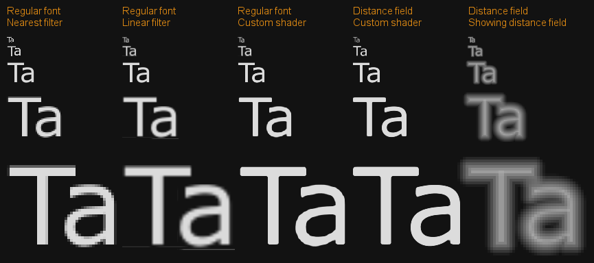
A common technique to deal with a similar issue in font-rendering, is to rasterize the font as a signed-distance-field (SDF), which also enables a bunch of other neat advantages, like outlines and variable thickness at no additional rasterization-cost.
To generate this SDF, we don't rasterize the font itself, but for every pixel store the distance to the nearest outline. If we're inside the glyph, we simply keep the positive value of the distance, if we're outside the font, however, we give it a negative sign.
As the texture is much more homogeneous around the critical edges now, biliniar interpolation will do a much better job and we can still achieve nice (even sub-pixel) anti-aliased borders by - rather than simply discarding interpolated pixels with values < 0 - applying a slight gradient to the alpha testing cutoff.
To apply this technique to our vegetation textures, however, isn't as straightforward as it may seem. Calculating the exact distance to an outline is somewhat trivial for vector graphics, but for raster graphics - like our vegetation textures - a few distinct puzzle pieces are missing: The textures may for example contain completely smooth alpha gradients and even if there are clear lines between transparent and opaque areas, the exact border may lie somewhere in between our discrete pixels.
Raster Graphics Signed Distance Field Generation
So, let's have a look at our fast implementation of generating a SDF from a raster-graphic's alpha channel:
Step 1: Upscaling
As we don't want to restrict the threshold-gradients to exact pixels in the target resolution, we first upscale the alpha channel - in our case, by a factor of four. Notably, we don't use bilinear interpolation for this purpose - but rather a more expensive interpolation method. In our case that's, Bicubic Interpolation.
This should be sufficiently large to combat artifacts introduced by stray pixels, as they have much larger areas to smoothly spread over in the upscaled texture.
Step 2: Applying the threshold
Now, we iterate over every pixel of the image taking into account the surrounding 3x3 area and perform the following operation:
Are all pixels in the 3x3 area < the threshold?
Then mark the center pixel as -∞
Are all pixels in the 3x3 area > the threshold?
Then mark the center pixel as +∞
Of all the values in our 3x3 neighborhood, are no pixels closer to the threshold than the center pixel?
Then mark the center pixel as 0
Otherwise: Are we < the threshold
Then mark the center pixel as -∞
Otherwise: (We are > the threshold)
Then mark the center pixel as +∞
This yields a rough starting point for our SDF as the resulting values are already in the correct range, so we copy the result to our upscaled-resolution SDF texture.
Step 3: Generating the SDF
To begin with, we generate a distance field around a singular point - this distance field isn't signed but simply contains the Euclidean distance to the center.
We will use this static distance field later as a lookup. In our case, the distance field is 33x33 pixels normalizing the distance factors to a distance of 33+1, as otherwise even the edge-pixels in all cardinal directions would end up as zero, making it effectively a 31x31 distance field.
Now, we iterate over all the pixels in our texture, again taking into account the 3x3 area around any given pixels (repeating at the edges) and perform the following operation:
If the center pixel is 0
We apply our pre-computed distance field to the SDF centered at our current pixel.
If all values in our 3x3 range are either +∞ or -∞
We leave the corresponding value in our SDF untouched.
Otherwise:
We average all positive or zero value positions from our 3x3 neighborhood and round them to the next integer.
Then, we apply our pre-computed distance field centered on this position.
To "apply" our pre-computed distance field lookup to the target SDF, we consider the fact, that the smallest distance to a border will be closer to 0 than any other border-distances can be to it, as otherwise they would've been the closest border.
Using this logic, we can iteratively update the "best" SDF value with closer and ever closer values until we've visited all gradients.
To turn our pre-computed distance field lookup into an SDF, we simply adopt the sign of the value that currently resides in the SDF onto our new offered distance, yielding:
Please note the cast to int16_t, as -(-128) is not representable in int8_t!
Step 4: Downscaling
Now, we can simply downscale our generated SDF by pixel averaging and bring the values into our expected output range (signed -128 ~ 127 to unsigned 0 - 255), yielding our approximate low-resolution output SDF.
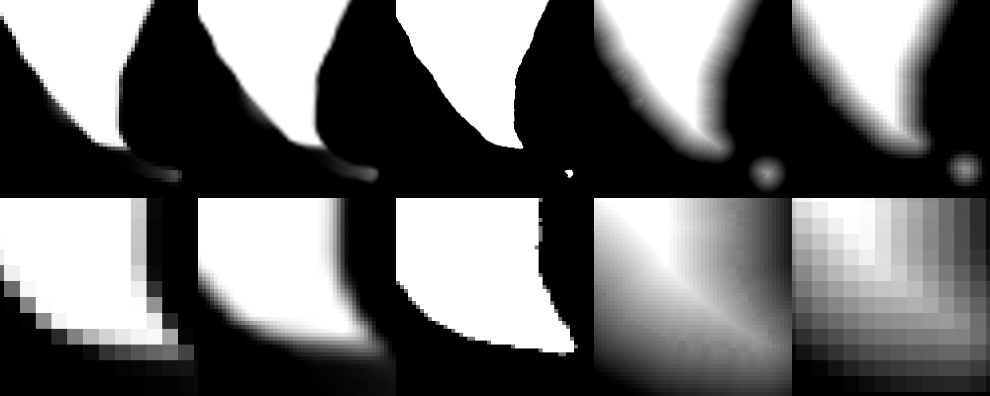
Here's a step by step view of how a particular segment of our alpha channel transforms through the algorithm described above:
Utilizing the Signed Distance Field Alpha Channel
Surprisingly, as we've already been using a hard threshold to decide whether a given pixel shall be discarded, the changes to make use of our new SDFs are rather minimal. We've previously been using our alpha-cutoff at 0.3, but as now our cutoff point has moved to the middle of the value range representing 0 as 0.5, the sole change that is required to correctly utilize the SDFs is merely this:
if (alpha < 0.33)
if (alpha < 0.5)
discard;
discard;
As blending would introduce nonsensical values into our G-Buffer, there's no need to do the threshold-widening anti-aliasing approach commonly used with font-renderers for our deferred renderer, hence no further changes are needed.
Visual Improvements
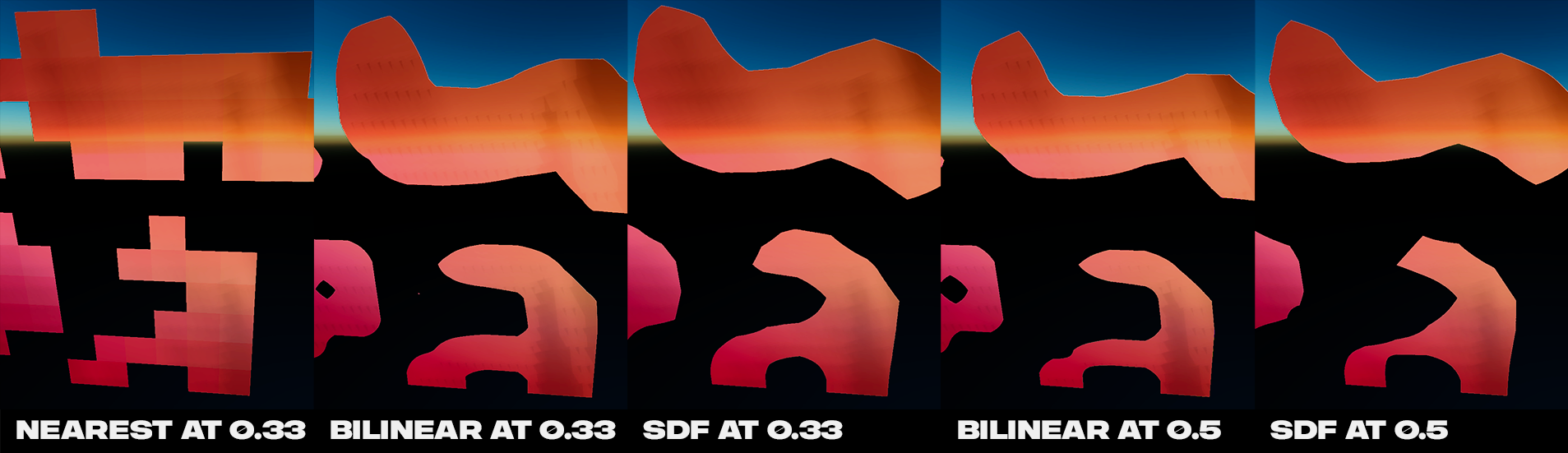
As the alpha "stepping" arises from bilinearly interpolated harsh alpha transitions, the differences (and issues) are much more pronounced with textures that exhibit large chances in value over only a few pixels, where with signed distance fields, the results become consistent across *all* textures.
That said, there is certainly room for improvements with generating our SDFs - but our results aren't meant to compete with advanced multi-channel SDF font rendering approaches, but rather to improve alpha outlines for vegetation rendering.
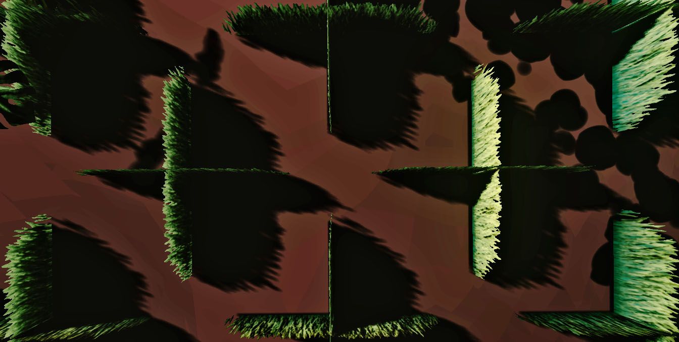
Leaf Shadows
The way light-shadows are implemented in traditional rendering pipelines is by additionally drawing the scene from the light's perspective into a depth buffer and then shading the screen-space view by reprojecting the world-space coordinates of the current fragment into the view of the light and comparing the depth inside the light's depth buffer to the depth of the current fragment. As this would result in terrible flickering on the shadow-casting surfaces (due to floating point inaccuracies) a bias is usually applied to the depth values retrieved from the light buffer, in order to slightly shift the shaded depth behind the shadow casting surface - hence keeping it in the light.
The problem with this approach becomes apparent, when rendering very thin geometry that's connected to another surface: Due to the slight bias term in the shadowing comparison, the backfaces of the surfaces would still remain in light. This itself is an easy fix, as computing the dot product between the light direction and surface normal allows us to easily discard surfaces, which can not possibly not be shaded, as they're pointing away from the light surface, however, The surrounding geometry will still only enter the shadowed region slightly after the shadow-casting objects position.
A step in the right direction: Light-View Offsetting
The culprit of the apparent disconnect of the shaded regions is the bias term, which shifts the shaded region away from the shadow's contact point. Simply adjusting the bias terms can reduce the the size of the disconnected region, but only at the cost of lit surfaces ending up with shadow artifacts.
Targeting just the issues with the contact shadow disconnects, we can therefore make the following change to the usual shadow rendering pipeline: When drawing the thin leaf geometry to the light depth buffer, we can slightly move the vertex positions of the relevant objects in the opposite direction of the light-source, so, in effect, pre-subtract of the bias term by slightly shifting the rendered geometry towards the light-source. This cancels out the bias term, reducing the disconnected region to zero.
Unfortunately, even though the issues with contact shadows have now been resolved, this creates a new problem (which is what the bias term was initially meant to solve): As the leaf-geometry now has been rendered at an altered position, which is closer to the light source, even the lit side of our leaf-geometry now firmly lies in it's own shadow.
Stepping out of its own shadow: Render-View Light-Space Offsetting
By separating out our thin geometry via a stencil bit, we can easily counteract this self-shadowing by adjusting the bias-term accordingly, but this still doesn't actually fix all of the artifacts, as one problem remains to be taken care of: Now, when leaves cast shadows on other leaves the contact points exhibit the exact same problem that we had previously encountered with the shadows cast from the leaves on other objects. Yet again the difference in the view and light rendered vertex coordinates becomes a problem that can't easily be overcome by just adjusting the bias without introducing other artifacts.
We obviously can't resolve this by also moving the view rendered vertex coordinates as that would undo all of the progress we've made so far and additionally result in a model position that differs from the one specified for the scene, but we can do something very similar. As we already have access to the world-space positions of each fragment when applying shadows, we can - before projecting the fragment positions into the view-space of the light - slightly move them in the opposite of the light-direction (so, towards the light) by the same amount that we've done so when drawing the mesh into the depth buffer of said light. This perfectly counteracts the difference in position, as now the light & view rendered light coordinates end up at the same position and we can simply use our default bias term to discriminate between lit and shaded faces, leaving contact shadows perfectly intact.
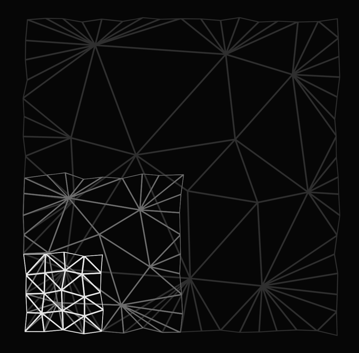
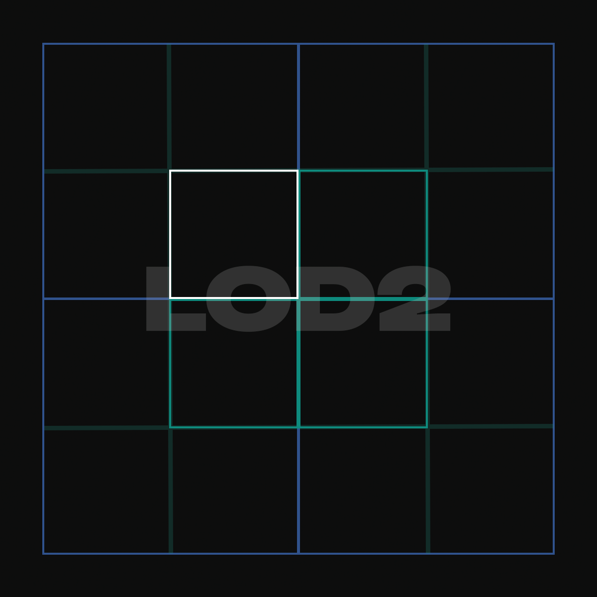
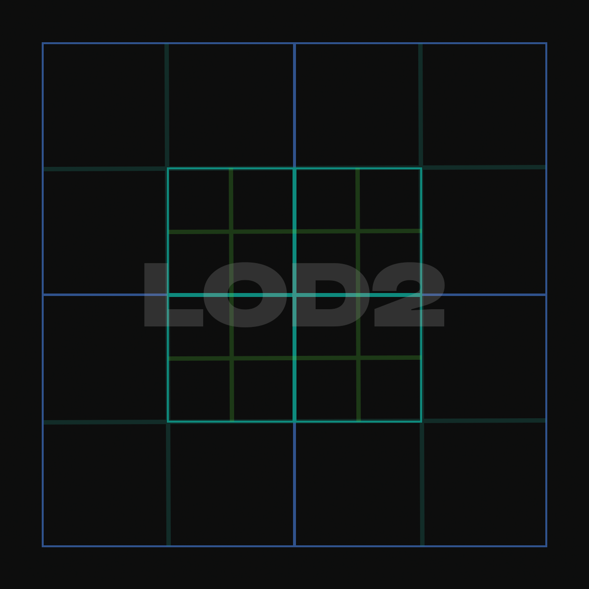
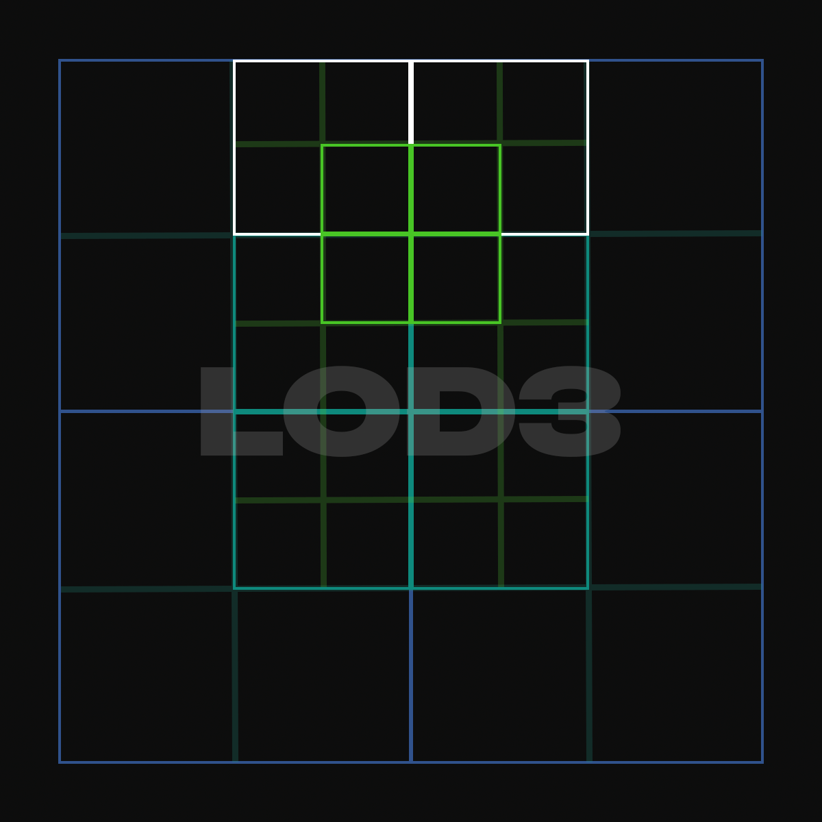
Smooth LOD Blending
For modern traditionally-rendered open-world games LOD (level of detail) switching is an essential mechanic by which objects which take up less space on screen are represented by lower-poly versions than if the same model were to be rendered up-close. For many objects the LOD transition (switching out one LOD for another, as the camera moves throughout the world and objects become larger or smaller on screen) can be done somewhat seamlessly, without any fancy techniques (as long as the low poly mesh accurately represents the higher-fidelity version from further away) - or even if not, the resulting "pop-in" effect usually occurs scattered across the screen wherever a mesh happens to pass the megic boundary into a different LOD, however, for dense vegetation (e.g. grass, flowers) - as this transition will continually occur at a consistent distance / position on screen, simply switching out LODs will quickly result in a very apparent transition-point, or a very high number of LOD transitions is needed to prevent this.
In order to tackle this, we can instead simply fade smoothly between different LODs. With a deferred rendering setup, this means that we need to dither between LODs, smoothly shifting the resulting likelyhood of pixel-rejection across the LOD boundary.
The implication of wanting to be able to fade between LODs is that both levels of detail of a mesh need to be loaded & (at least partially) rendered (wherever fades occur), so, simple LOD switching aims towards linear effort to render a model at any given distance (with the complexity of the mesh increasing the more space it takes up), but with fading LODs, the effort to render a model would naively be highest when transitioning between displayed levels of detail.
There is, however, some trickery we can perform, in order to at least reduce the complexity of rendering models in transition...
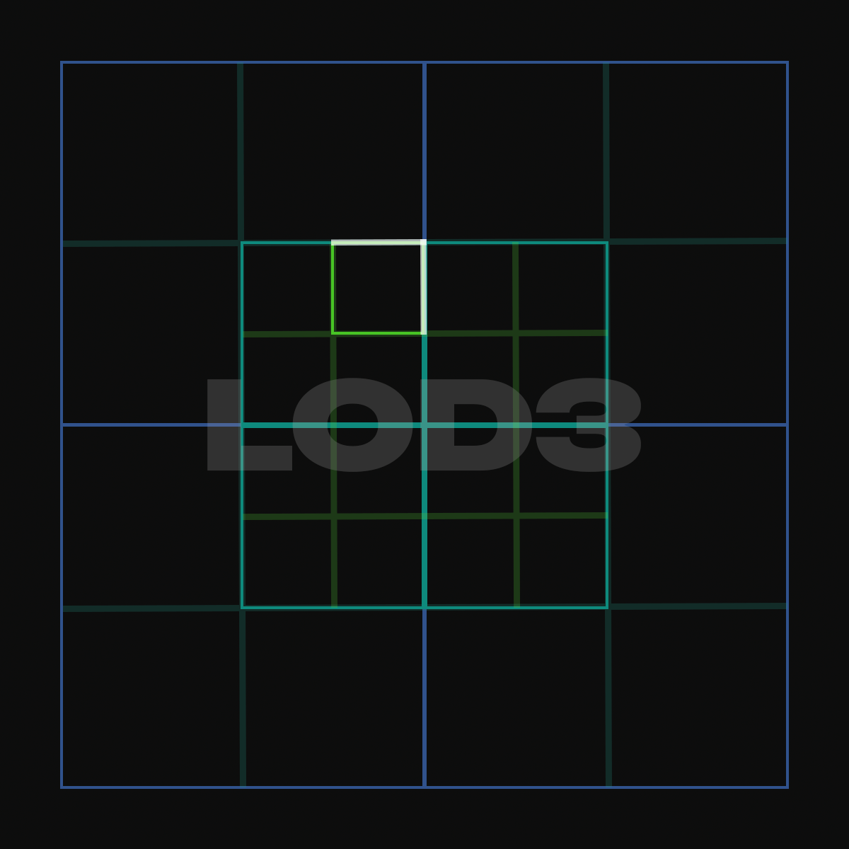
Distance-Aware Geometry Shader Triangle-Rejection
Our Vegtation-LOD architecture provides each object with a minimum and maximum renderable distance, expressed as a LOD-transition point index - hence, they always occur at pre-calculated distances which can be retrieved from a set of lookup-tables for the fade-in & fade-out distances of any given LOD-transition-point (they actually contain the squared distances in our implementation to speed up the comparison, but that's besides the point).
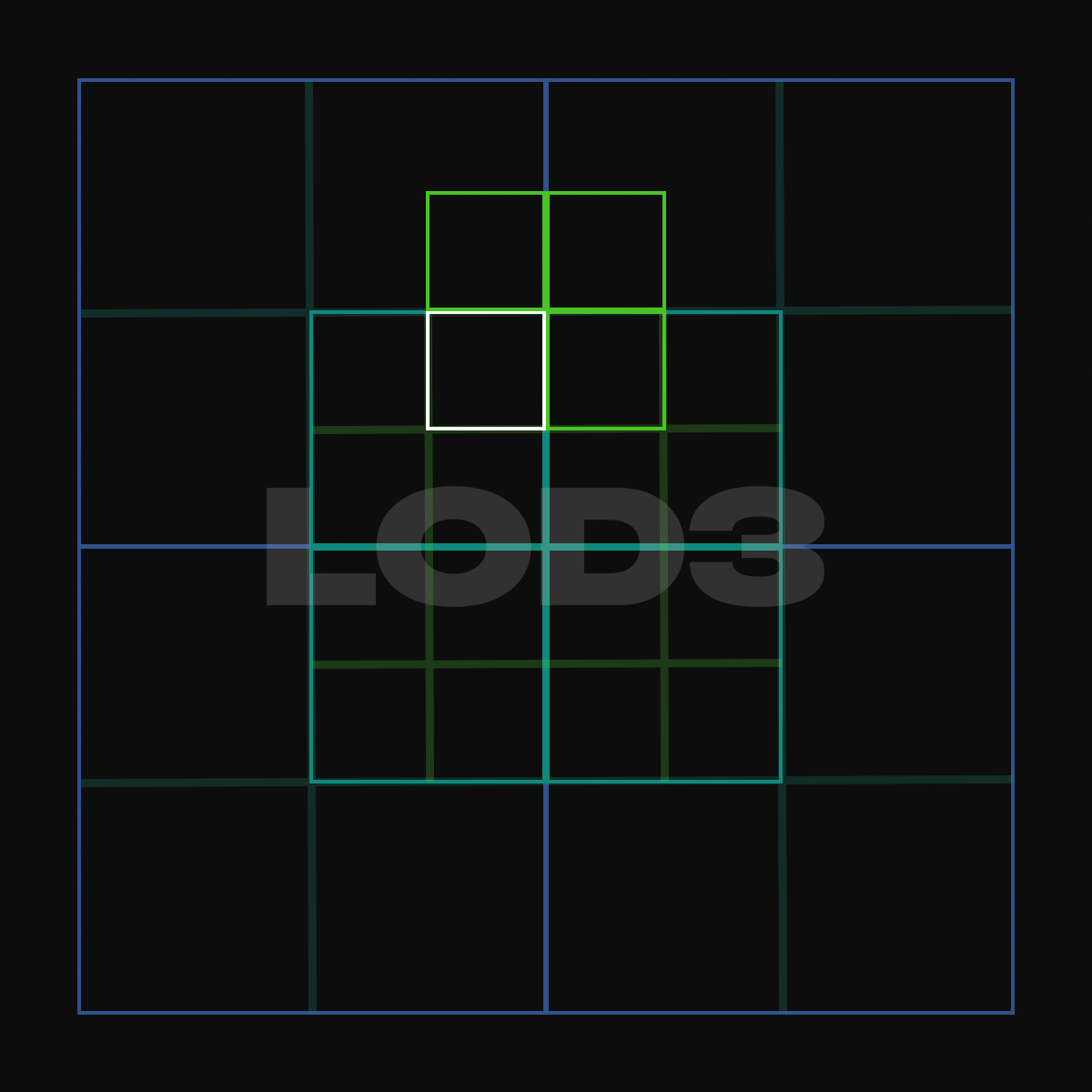
Now, when we arrive in the geometry shader for any given triangle, we can easily determine if any of the vertices are within the set bounds of our corresponding LOD-regions (or some are behind the visible LOD area and some are in front - to handle triangles spanning multiple LOD regions) - if they fail this check, we can simply reject the triangle outright (by returning without any calls to EmitVertex or EndPrimitive), excluding it from any further processing.
This leaves us with the triangles that are either fully visible or within the blending region. For each vertex of those triangles we can now calculate the fadeInFactor of the first LOD region and fadeOutFactor of the last LOD region. Those fade factors are now valid to be interpolated barycentricly into the fragment shader.
As meshes may span multiple LOD-barriers we have to consider even & odd transition boundaries separately, as - depending on which side of the LOD-barrier we are, when entering a blending region - we need to either keep or reject the fragment with a gradual increase (or decrease) of rejection likelyhood the further we step into the transition region.
This leaves us with nicely transitioning vegetation meshes. The same principle can easily be applied when meshes are rendered into light depth buffers to achieve matching smoothly interpolating LOD shadows (the camera position to calculate the world-space vertex distances from does not become the light position here, but remains as the player camera position).
Vegetation LOD Architecture
Using meshes with different levels of fidelity to represent the same object is a common technique in modern rendering engines (usually referred to as just LODs). However, this doesn't translate nicely towards a generic vegetation rendering system, as e.g. a field of singular grass bushes would preferrably be represented by one big grass billboard from afar, and whereas the individual leaves of trees may be relevant up-close they're certainly not individually relevant from afar, but should rather be captured by a larger mesh representing all the leaves (at least of a singular branch) - and eventually even the entire tree should be able to merge into a singular billboard.
One would assume, that this means that vegetation LODs can at least be hierarchical - so that a tree would be anything from a billboard to a high-fidelity model with each leaf & branch being represented by detailed meshes - which is possible, but certainly not desirable:
Firstly, it would mean that for each kind of tree, only one configuration of branches and leaves would be the legitimate high-resolution representation (which would be either very inefficient, or very boring), but also - an example that represents the problem in more severity - if we have a meadow that spans an area including a sharp cliff, we can't place our mega-grass element at the top (as otherwise the high-fidelity version would not have any grass at the bottom of the meadow) nor at the bottom (opposite problem) nor in the middle (not correct in any case).
This means that our vegetation LOD Architecture needs to consist of separately specified levels of detail, to allow maximum flexibility for tree configurations and complex landscapes. And - in order to make separation of LODs by distance possible, individual elements need to allow specifying maximum and minimum levels they match with (in order to not require splitting up large meshes when they get too close, but are perfectly sufficient in detail even at a distance). This can be further improved by adding the option to support "spawning" lower LODs from arbitrary LOD levels at known starting points, to reduce duplication of common mesh arrangements.
Shared Texture-Streaming Architecture
Adding vegetation objects as a separate entity type to render objects into the engine - as they require different types of attributes to be associated with the models - leaves us with a challenge:
Our existing texture-streaming architecture is currently targeted towards gathering only render object textures (and updating the corresponding gpu resources pointing to them), but it wouldn't make sense to entirely duplicate this functionality for vegetation objects - and unifying the behavior across different types also scales much better with adding even more different types of rendered objects in the future (it also allows for using a single texture across different types of objects).
Resource Loading Journey
To illustrate the process, let's have a look at the different stages which need to be completed before a texture can be rendered to a certain type of rendered object:
A Chunk with different types of render objects is added to the renderer
Basic information about the associated meshes is retrieved (Extents, Mesh File ID, Texture File ID, etc.)
The data-chunk with generic information is uploaded to the GPU
When the upload is completed, the chunk can be forwarded to the culling compute shader
If a certain bounding box is considered visible by the culling compute shader, it's associated object's visible counter will be incremented (for the relevant LOD, if applicable)
On the next frame the CPU-side iterates over all elements contained in the pools of all rendered object types, finds the ones that are unloaded, but have been referenced on the GPU side and enqueues them into the "Please Load" queue. The objects are now marked as "requested"
If load-capacity is available the request for the corresponding model & texture is enqueued to the asset-query system
The model or texture is asynchronously loaded from disk, decompressed & converted to a usable format
The asset-query handle is checked for completion, if completed, the resources are collected by the renderer-streamer
The required resources are allocated for storing the asset on the GPU
The Asset-Data upload to the allocated resource is enqueued, and the corresponding upload-handle is associated with the rendered object / texture data
When iterating the objects at the beginning of the frame for unloaded visible objects & the "requested" flag is set, we check if there's an associated upload handle and check for upload completion
If the resource is a texture and the upload is completed, we register the new texture (with the associated texture sampler) in our bindless texture array
We then update the object's reference to no longer point to unloaded texture / mesh data, but the newly loaded resource.
Now, when the cull compute-shader finds those instances to still be visible (whose objects now point to loaded resources), it creates draw calls for each of the matching instances
Finally, the meshes are drawn to the screen with the freshly loaded mesh & texture data
Request States
For textures specifically, this means that - from the perspective of the renderer-streamer - we can split the asset loading process into two phases with various sub-states each:
CPU Load Request
Awaiting an Asset Query Slot
Awaiting Asset Data from a running Asset Query
Alternatively: Awaiting Completion of a different CPU Load Request (created by a different object, but using the same texture)
Ready (the request will continue as a GPU Update Request)
GPU Update Request
Allocating the Texture
Enqueueing the Texture Upload
Awaiting completion of the Texture Upload
Setting the texture to the Bindless Texture Array
Setting the Texture Array Index to the Objects (making it available to the renderer)
State Handling
With this rough overview of the procedure of loading textures in mind, let's consider the following cases and how they're being handled now in a bit more detail: (Steps performed as part of the asset-query subsystem are displayed with reduced focus)
A newly loaded object requires an unloaded texture
In this case, we simply follow the steps detailed above:
Enqueue Texture asset request → dequeue → forward request, store handle → process request → load asynchronously → mark ready
Update entry in the Render- / Vegetation-Object Pool with the bindless texture array index
A newly loaded object requires a texture which is already requested
Store a dependent texture request with the type & index of the corresponding object
Every frame, we check if the underlying object has advanced its state from "Waiting for Asset Request"
If the Object has been advanced, we enqueue our GPU Update Request pointing to the upload handle
When the upload has been completed, if the texture hasn't been set to the Bindless Texture Array yet, we perform this ourselves (can happen if uploads complete whilst iterating GPU Update Requests)
Finally, we update the corresponding entity in the associated GPU object pool to point to the index in the Texture Array
A newly loaded object requires a texture which is already uploading
We merely need to insert a GPU Update Request for the corresponding object
When the associated upload handle has been marked completed, if the texture hasn't been set to the Bindless Texture Array yet, we perform this ourselves
Finally, we update the entity in the associated GPU object pool to point to it
A newly loaded object requires a texture which is already available
Here, we only need to update the object's entity in the associated GPU object pool to point to the corresponding index in the Bindless Texture Array
Rendering Soft Shadows
Achieving Soft shadows with traditional rendering techniques is far from being an accurate depiction of such phenomena in ray-traced scenes, but still significantly improves the overall look of the final output. Whereas soft shadowing in ray-tracing is an inherent property of tracing towards the larger surface of the light fixture, with a traditional rendering pipeline, there is no direct equivalent of this.
Experimenting with sampling the light fixture area over multiple frames and accumulating the result in screen-space has proven tricky, so usually simply accumulating the shadowed-ness of neighboring shadow-map texels is being used for a smoother overall look - but it doesn't come with all of the "real" properties of soft shadows, such as softness increasing with distance from the shadow-casting object. These things can be mimicked though by manually increasing the sampling radius depending on the depth difference between world-space and shadow map.
For sub-texel blending, we can simply subtract the fractional sub-texel position from the sample offsets and throw those positions into a weighting function, then accumulate the weighted samples and divide the sum by the combined weights.
In order to decrease the number of required samples per pixel, we begin by casting a sparse but wide net of shadow samples. If the accumulated result is partially shadowed (so neither all, nor none of the samples are fully in shadow), we collect more samples to resolve the full quality soft shadow.
To determine the smoothing range to be used for distance-based shadow penumbra sizes, we gather the average depth difference from the initial net of shadow samples, use that to interpolate between the minimum and maximum smoothing radius and use the inverse of the resulting value as bounds for our weighting formula.
float calculate_weight(vec2 offset /* = sample_offset - subpixel_offset */, float inverse_radius)

{

  float r = length(offset) * inverse_radius;

  r *= r;

  r = max(0.0, 1.0 - r * r);

  return r;

}
Temporal Global-Illumination Accumulation via Reprojection
Anti-Aliasing is commonly implemented via temporal multi-sampling and reprojecting previous frames into the current view-space in modern rendering engines. However, the same techniques can be adapted to combat the rough surface ray-tracing noise by accumulating and bluring ray-traced Global-Illumination samples over multiple frames. As we're tracing into a voxelized version of our rendered scene, we can additionally apply a morton sequence to our voxelization offset positions, to further improve the visual quality of the reflected geometry.
As there's quite a bit of overlap, it's very convenient to combine the GI accumulation with the application of Temporal Anti-Aliasing, as e.g. the color and depth differences observed in one, can aid the blending in the other. Unlike the TAA-pass, however, GI is meant to blur on a much larger range in both time and space, as the voxel-traced samples are much more unreliable.
That's why we take a blurred version (restricted by depth differences) of the previous frame as the starting point of the current one and also allow neighboring samples from the current frame to be included in the final color of the current frame's GI as well. That way, GI can slowly "bleed" across surfaces, merely inhibited by stark differences in depth curvature (= edges) between the surrounding samples.
There is, however, one complication to consider here: Global-Illumination sample color is inherently linked to the albedo surface color of which it had been reflected, so without accounting for this surface textures will get very washed out and blurry, as their final color is indirectly influenced by the neighboring texels via their contributions to the blurred GI sample colors.
To combat this, we remove some of the textural information from the GI data, by simply dividing the accumulated GI color by the current frame's albedo color (offset by some constant, to limit the negative impact of incorrectly attributed samples) before storing the final accumulated sample. When referencing this accumulated GI texel during the next frame, we'll obviously have to re-apply the albedo color, before combining it with the newly acquired sample.
It's important to not fall back to the shaded output color here, but rather use the raw albedo color, as otherwise directional differences in shading would have an enormous side-effect on the accumulated Global-Illumination samples.
Another point to consider is that GI samples inherently cannot be interpolated between texels, as otherwise surface information from one surface may bleed into an unrelated other surface through such means.
The Troubled Seas of Voxel-Field Tracing
In contrast to ray tracing against lower poly versions of the rendered scene, where flat surfaces can trivially be represented accurately, there are additional complications with such areas as soon as such surfaces are rasterized to a grid that doesn't exactly conform the directional preferences of the surface plane.
First of all, when resolving from the world-space position in the rendered output to the voxel grid position, we may land inside or potentially even behind the voxelized equivalent.
Secondly, as flat surfaces that don't align neatly with the voxel grid, will inhibit at least some stair-stepping, we could - especially at extremely shallow viewing angles - accidentally encounter a ray intersection with the same surface, by running into such a stair-step.
Lastly, when tracing staring from a voxelized corner position, we may accidentally run into the voxelized remains of a close surface that lies in an irrelevant direction, which occupies our path by simply being too close to the origin surface.
To combat these points, we firstly offset our voxelized position in direction of the current surface normal. If we're still stuck inside a voxel at this point, we allow the voxel tracer a couple of steps through solid voxels, until we'd give up and assume the target voxel to be occupied.
This helps to achieve much more pleasing results than simply doing one or the other, as those factors combine nicely to combat the issues mentioned above pretty convincingly in all but exceptional edge-cases.
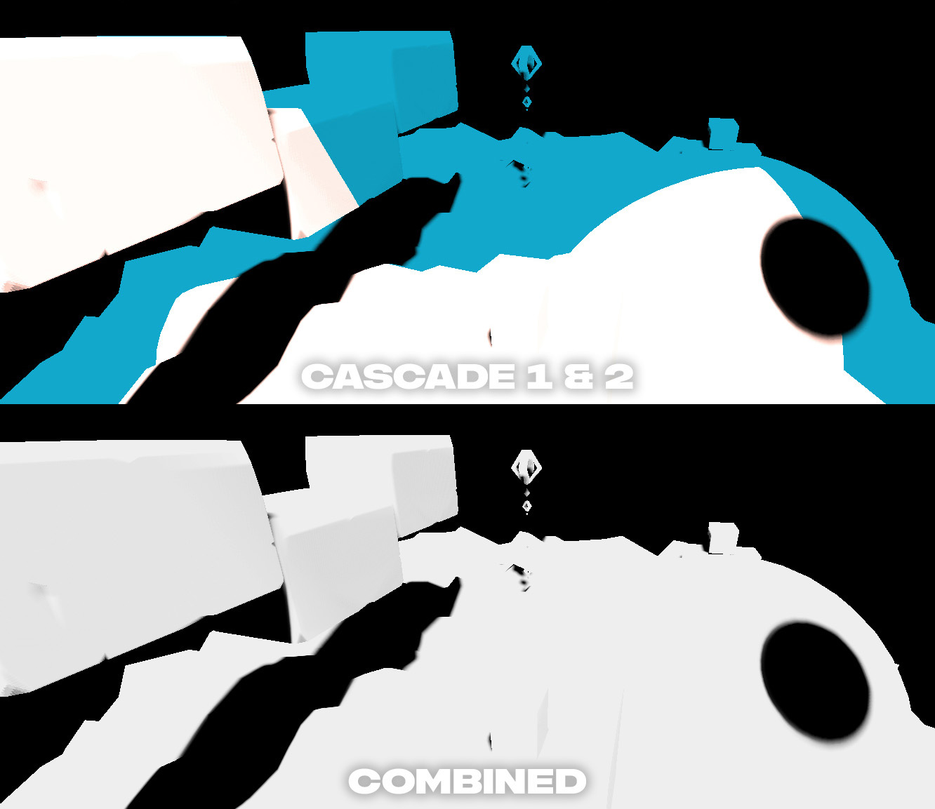
Cascaded Shadow Maps
Rendering sun shadows usually comes with a bit of a trade-off: As texture-resolution is limited, shadows may either be high quality, but fade out very quickly, or they fade out much futher away, but are much less detailed.
As a solution to this conundrum, which stays within the traditional rendering pipeline, we can simply render the world from multiple increasingly large orthographic views (biased towards the look direction). This results in having a view with high quality shadows for close-up detail, but also far-reaching shadow map coverage (with lesser quality where it matters less).
When applying the shadows to our scene, we can simply iterate through the list of our so-called cascades, until we end up in-bounds of the light matrix. This is handled as usual, we simply project the world-space position of our fragment to the view-projection matrix of the corresponding shadow-map and end up with a view-space coordinate into the associated texture.
In order to obscure the transitions between the different shadow-maps, we can employ a simple edge-fade, smoothly transitioning from one cascade to another.
for (; layer < 4; layer++)

{

  // decoupled matrices, otherwise `lightSpacePos` can be calculated from the previous one

  mat4x4 lightVP = lights[lightIdx + layer].vp;


  vec4 lightSpacePos = lightVP * vec4(worldPosition, 1); // world position in light space

  //lightSpacePos /= lightSpacePos.w; // not needed, orthographic!


  float maxPos = max(abs(lightSpacePos.x), abs(lightSpacePos.y));

  if (absMaxPos < 1) // if not out of bounds: stop!

    break;

}
Renderer Architecture: Occlusion Culling
As we're generating multi-draw-indirect-buffer for rendered chunks from a compute shader, we'd like to reduce the number of objects being rendered to only consist of what's actually visible on screen.
One such approach is Frustum Culling - a simple technique, which attempts to reject objects behind or next to the View Frustum. It's fairly cheap and easy to implement - simply requiring a bounding box to be projected to the screen, but it's also inherently limited, as it can't combat overdraw.
struct gpu_lod_obj_info

{

  gpu_lod_info lods[MaxLodCount]; // vertex, index buffer offsets, index count, request counts per LOD

  vec3f maxBoundingVolume; // maximum dimensions of all LODs

  uint32_t validLodMask; // bitmask of lods available to be loaded

  vec3f centerOffset; // combines with `maxBoundingVolume` to a bounding box of all LODs

};
A more intricate and powerful technique is called Occlusion Culling. Here, we attempt to compare the depth of the projected object or bounding box against a reprojected depth buffer from the previous frame (which may additionally include some static close objects being re-rendered on top, to combat gaps in the reprojected depth buffer).
To make those lookups cheaper, we can construct a mip-chain from the depth buffer, which contains both the minimum and maximum depth value of the represented depth-buffer values (as a best- & worst-case depth). To make using this mip-chain much more straightforward (as we can't just assume that it's valid to split a certain texel down the middle and end up in the right place of the next mip), we can simply restrict the reprojected depth map size to the highest power of two in x and y less or equal to the depth buffer resolution.
Now, with the help of this depth buffer mip chain, we can easily check if the worst case depth of our object - so the closest it could possibly be, derived from its bounding box - can even occupy a certain area on screen (as opposed to being behind some other static object from the reprojected depth).
If our object's worst-case depth lands between the minimum and maximum depth represented by a certain mip texel and is at the edge of the bounding box, we can recursively check if the data stored in the underlying mip's texels makes this decision more obvious. Otherwise, we have to draw the object on screen.
Renderer Architecture: Objects & LODs
To achieve fully GPU driven render object streaming and for some significant throughput advancements, we'd only like to stream full chunks of static render objects to the GPU as a simple list of render object instances to generate a lodded multi-draw-indirect-buffer.
New chunks are simply supplied to the renderer as a list of such render object descriptors (position, rotation, scale). As the descriptors need to be able to look up information about the corresponding render objects, common to all render object instances (bounding boxes, vertex & buffer offsets, etc.), we want this lookup to be a simple index lookup on the GPU side, we allocate space for each distinct render object into a pool of Render Object Information.
struct render_object_instance

{

  uint32_t id; // renderer turns this into a pool idx

  vec3f pos, rotationAngles;

  float scale;

};
Now, for every chunk the compute shader which generates the multi-draw-indirect-buffer is called once, with the offset and size of the corresponding list of render objects.
Here, we can now do all sorts of culling operations and determine the correct LOD to be used for this draw-call.
GPU driven LOD streaming
So far, we've simply assumed, that all LODs have been loaded and are available to the compute shader. However, we most likely don't even wanna stream in all of those LODs - at least in most cases.
By simply adding a requestCount to our Render Object Information for each object, we can simply atomically increment (can also be weighted by importance / size) whenever an LOD is being requested or drawn.
After each frame the CPU-side iterates over the occupied slots of the pool, finds the missing LODs with the most requests and forwards it to the asset-streaming subsystem, which will asynchronously read, prepare and upload the LOD's mesh data to the GPU. Prioritization is handled via the requestCount.
As even loaded LODs are marked this way, the unloading of LODs can be handled in a similar fashion. Obviously, the requestCount needs to be reset after every frame.
struct gpu_lod_info

{

  uint32_t vertexOffset; // offset into the vertex mega-buffer.

  uint32_t indexOffset; // offset into the index mega-buffer.

  uint32_t indexCount; // number of indices to be drawn; 0: not loaded.

  uint32_t requestedCount; // number of draw requests during the last frame.

};
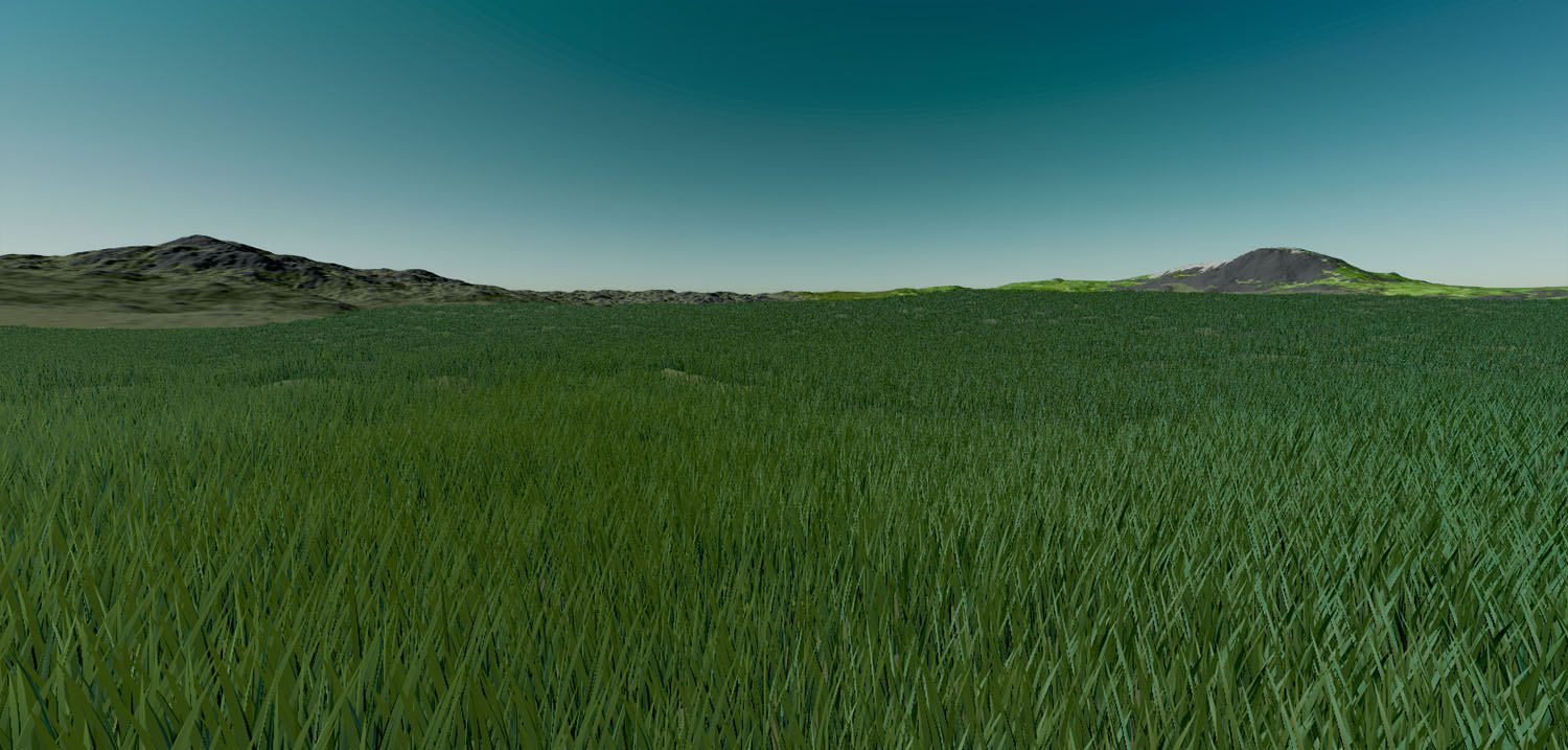
Vegetation Rendering
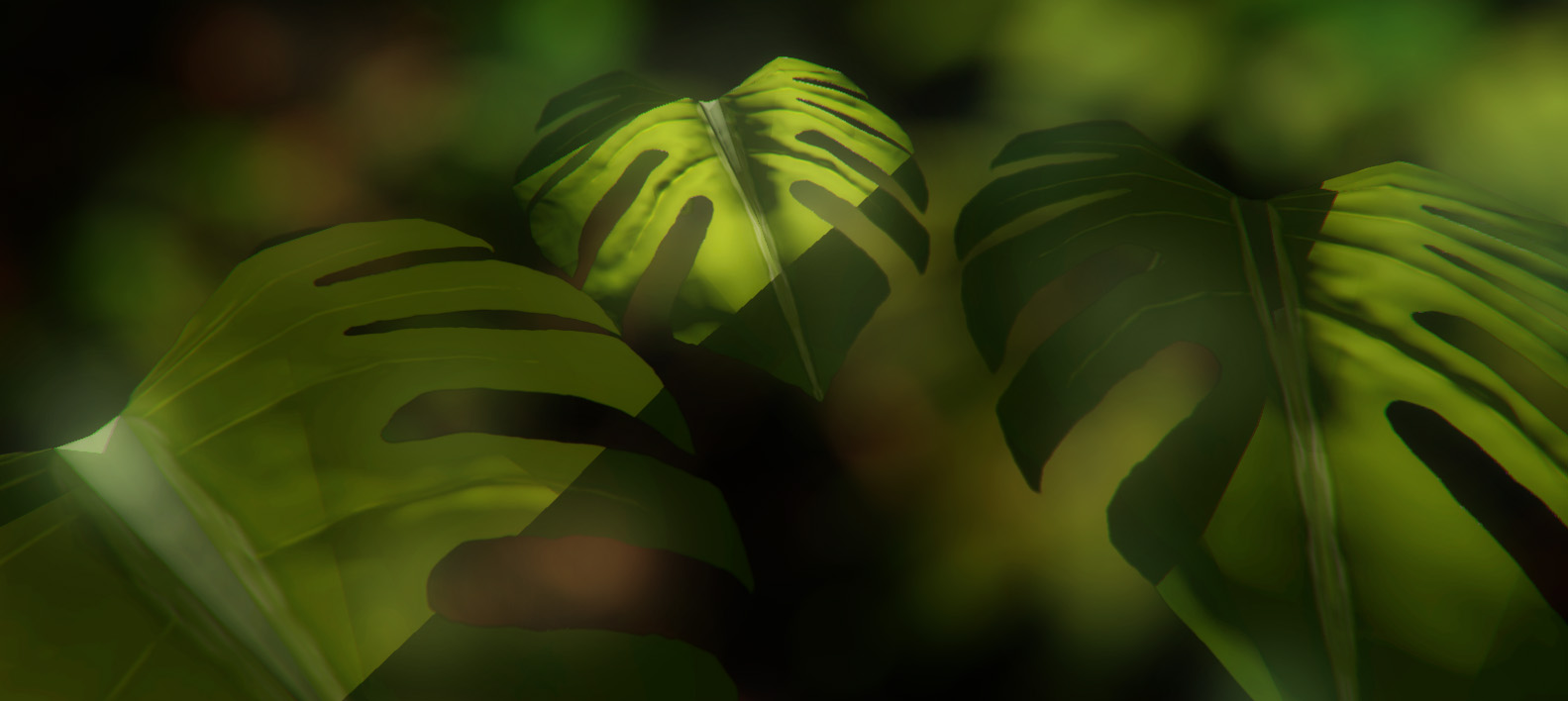
Although vegetation may be very complex to portray accurately in a real-time rendering engine, there are a couple of different factors, that combine to give a relatively cheap, but still somewhat realistic impression of actual plant behavior. Tree trunks might be able to get away with relying on good rendering fundamentals, branches might be happy with the first two components, but especially large leaves require a whole set of tricks to achieve a convincing look. So, let's go step-by-step, from basic to specialized.
Good Fundamentals
As already mentioned, good fundamental rendering techniques can already carry some of the weight when dealing with large pieces of vegetation: So, normal-mapping, shadows and physically based rendering from other parts of the rendering pipeline are also very useful here. Normal-Mapping specifically is crucial to the look, mimicking complex geometric detail on the comparably flat surfaces of leaves and bark of trees.
For this demo, we've merely applied normal maps and simulated a linear block of shadow, as this wasn't too distracting from the overall picture when trying to experiment with the more specialized components.
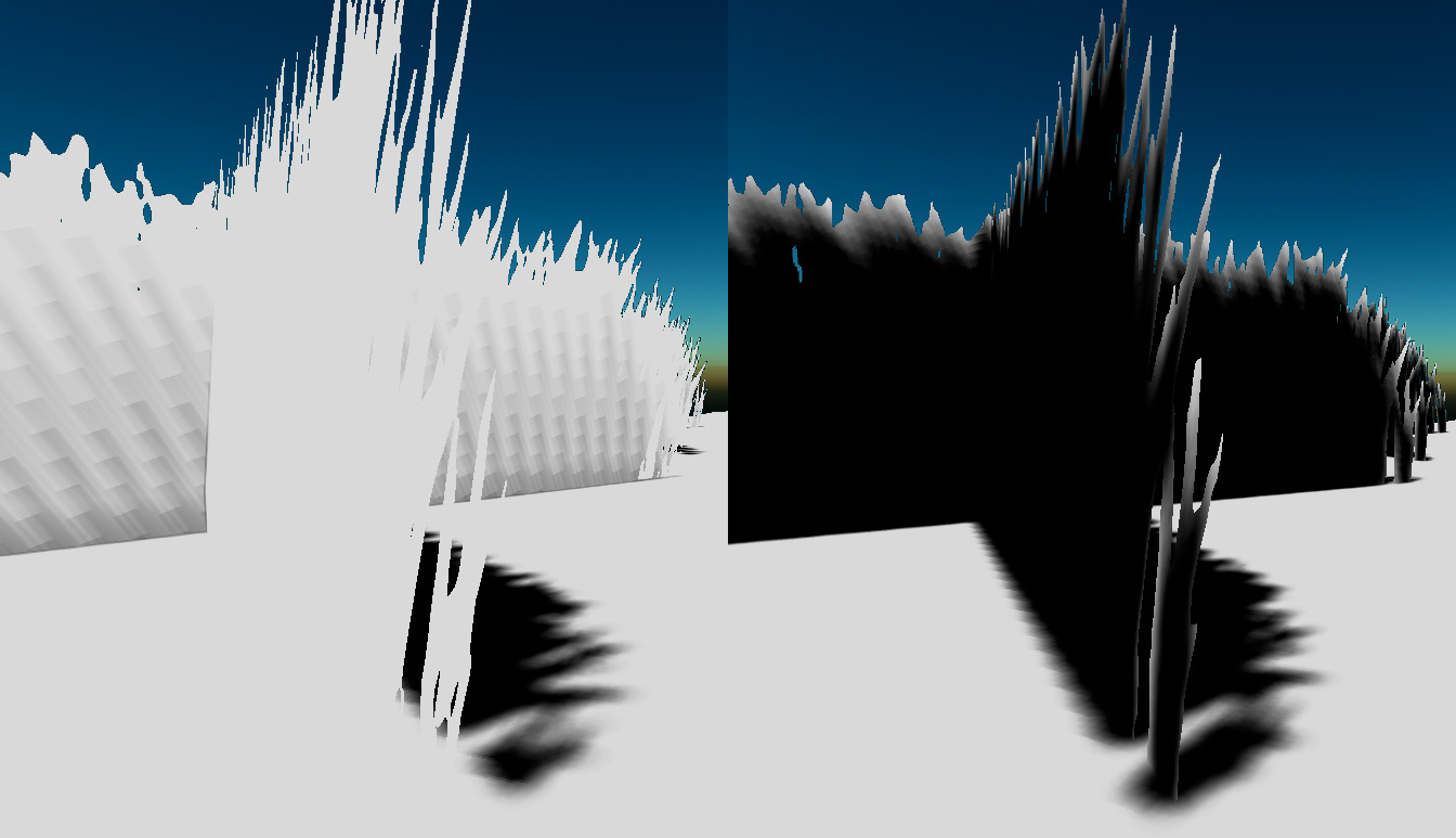
Wind
Now, a concept that's relevant for all but the thickest tree trunks - especially leaves, twigs and smaller branches - is the property of swaying in the wind. To achieve somewhat realistic swaying behavior, every vertex data contains - apart from positional and normal vector information - a weight, representing how impacted the vertex should be by the local wind vector (global wind vectors will look too uniform over a large scene and break the illusion fairly quickly). If an area touches - or is very close to - the ground, the vertex weight is zero (we don't want vegetation to be floating around, whilst penetrating the ground!), and for the thinnest tips of leaves the weight is one.
For branches it may be sufficient to simply apply the wind vector directly, whereas for larger leaves it would be ideal to take the overall "springyness" of the leaf and the leaf-internal forces into account. This will (hopefully) be explored further in the future.
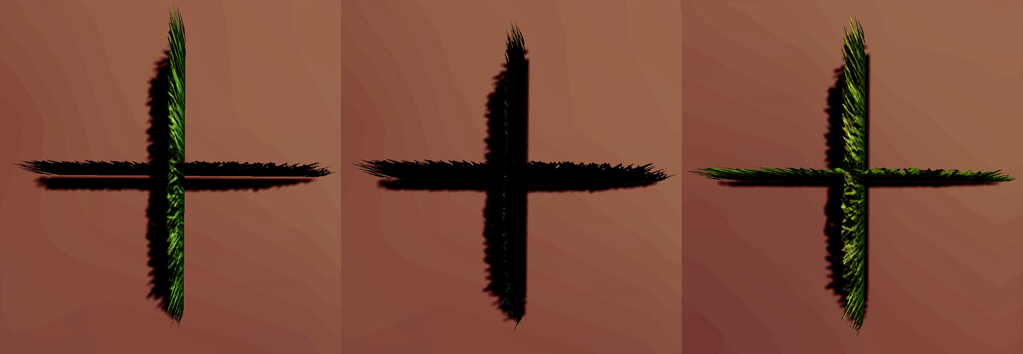
Backside Shadowing
As leaves are usually very thin, so, when viewing the unlit backside, we'd expect to see the light & shadows pass through the leaf structure to the other side. Thankfully gl_FrontFacing makes quick work of distinguishing between the front & backside, so we can simply flip the surface normal on the backside.
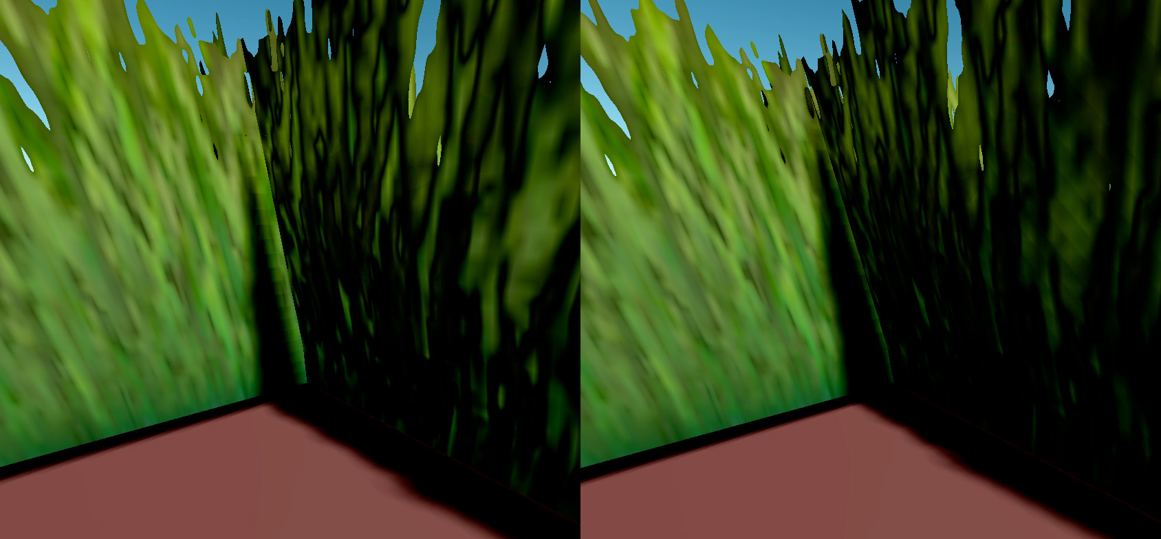
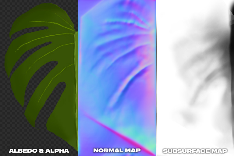
Subsurface Density
Lastly, leaves obviously have varying depth & density from the various veins passing through the leaf - even though we're simply representing the leaf with a bunch of flat planes. When viewing the leaf from the backside, we can derive our coloring based on this subsurface density and if the backside is being lit, alter the color of the light passing through the leaf to be darkened by the subsurface map.
Shader-Level (Bi-)Tangent Vector Calculation
Going on a slight tangent (😉), in order to apply normal maps to our vertex normals, we need tangent and bitangent vectors for our normal. These are commonly precalculated and stored alongside the other vertex data, but - as they can simply be calculated from the texture coordinate & world position of a mesh - they can also be calculated in a shader.
Geometry Shader (Bi-)Tangent Generation
As the tangent & bitangent vectors are identical within each triangle, they can simply be generated in a geometry shader from the world position and texture coordinates as follows.
For the sake of completeness and to validate, that our results are correct, we may also calculate tangent & bitangent vectors per fragment. Assuming decent occlusion culling, this is gonna result in a lot more work, as the same values will be generated for each fragment within a triangle.
Binary Serialization via Type-Seggregated Buffer Compression
In order to serialize generated assets into a custom model format, we need a minimal, fast & adaptable (de-)serialization API.
As discussed by gaffer on games, in order to achieve single-function de-/serialization per object, we introduce a similar API with a custom serialization-context input parameter.
      ERROR_CHECK(io_value(context, self.verts)); // list of vec3f

      ERROR_CHECK(io_value(context, self.triVertIndices)); // list of uint16_t

      ERROR_CHECK(io_enum_as_int(context, self.mirrorAxis)); // enum
Our serialization context now collects values of different types into separate arrays and when reaching the end of the stream, we can simply RLE-compress, Reference & Integer-Encode (where applicable) all the collected values per type to get a significantly reduced output size. By collecting symbols on-the-fly into a recent, approximate common and most-frequent buffer (upgrading values inside those buffers as we collect them), we can further improve our ease of referencing common values (although, this process is fairly costly upon decompression as well). Rather than just immediately encoding the symbols in a bitstream (which isn't even possible with rANS), we can gather symbol-frequency statistics over the generated symbols into histograms & use those to entropy-encode the symbol stream.
Afterwards, the collected symbols can be written to a file-/memory-/network-bytestream of our choosing.
Further improvements may be achieved, by meta-compressing the type specific symbol streams, in order to possibly combine commonly succeeding symbols into a separate meta-symbol, etc.
One of the limitations of this approach, is that all values need to be collected first (need to reside in RAM at once, rather than being able to be streamed in & out concurrently), and can only be compressed afterwards. However, following a data-oriented approach, this is usually a faster way to do this (compared to the constant context switching of compression & structure descent) and presumably results in a much simpler implementation.
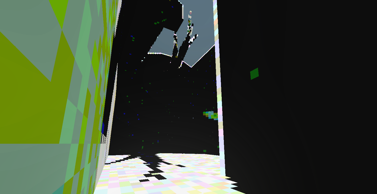
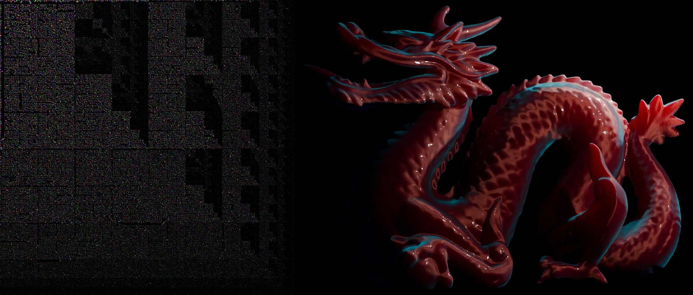
On Noise Patterns
When having a look at our original global-illumination implementation, there was a large amount of sporadic noise, that didn't result in visually consistent and seemingly smooth lighting. The noise source for this implementation had been a white-noise texture, that was being read at locations tied to the screen and world position & was being offset by a random vector for each frame.
Fully random noise (white noise) may lead to long-term convergence to the average, but not necessarily to a stable look over the short term, which is why usually blue (or even custom spacio-temporal) noise is used for such purposes.
This may lead to a more "patterned" looking noise texture, but also to a much higher rate of convergence to a visually consistent state.
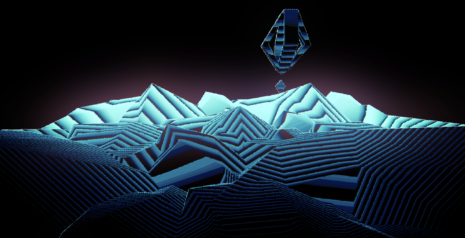
Voxel Traced Reflections
As global-illumination rays are cast in the deferred section of the render loop, we have access to roughness information associated with the surface of the first bounce. When encountering shiny surfaces - if we're fully respecting and considering surface properties - this can lead to some nice voxel traced reflections. On a per-frame basis, these reflections clearly display the resolution limitations of the voxel grid, although by jiggeling the voxel grid offset slightly over time, one could achieve a much smoother look (as we can observe in a future article). Unfortunately the limited (but also time-dithered) color accuracy is quite obvious here, as we haven't overhauled the noise pipeline on that end yet.
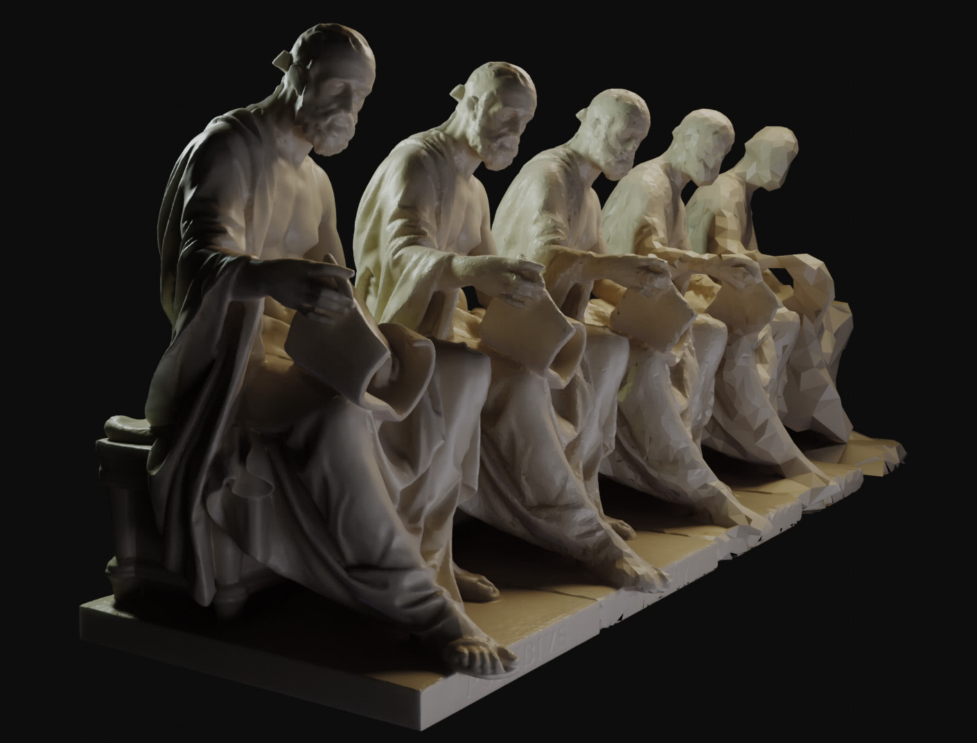
Comparing Triangle-Collapse and Edge-Collapse
Sadly, Vertex-Elimination is too limited to really produce any interesting results with reasonably high-poly meshes, as it's decimation floor is relatively high for any given mesh. So, let's only have a look at how Edge-Collapse & Triangle-Collapse fare on some more complex models and what their characteristics are when pushed to their limits.
Triangle-Collapse
Edge-Collapse
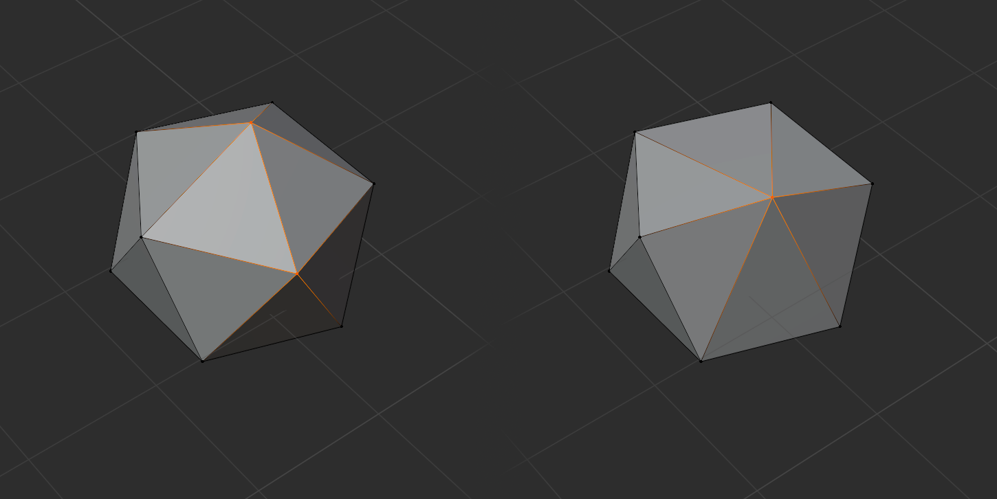
With the bottom plate we can clearly see how Triangle-Collapse quickly starts eating away even at large overall shapes. In order to get this under control, more "globalist" error metrics would need to be employed - but Edge-Collapse would most certainly similarly benefit from this. On the other hand, this is actually the only case where Edge-Collapse also ends up damaging normals (by flipping the triangle vertex-order). Still, it's far less pronounced as Triangle-Collapse. Ignoring all the issues, I think I prefer Edge-Collapse here over Triangle-Collapse, as it resulted in much smoother looking decimation. I expected the thin paper geometry to cause issues, but this fortunately didn't occur.
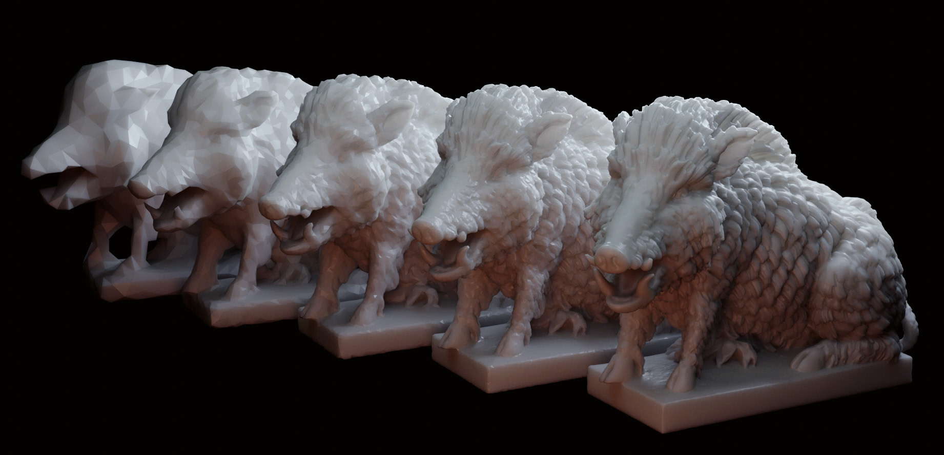
Triangle-Collapse
Edge-Collapse
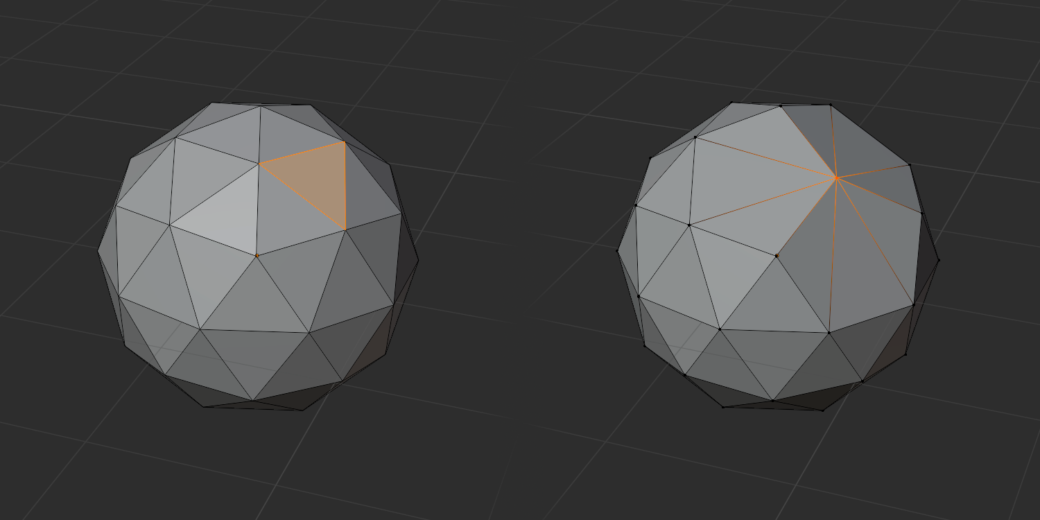
Here we can observe how Triangle-Collapse slowly arrives at an increasing number of problematic cases, where normals are accidentally flipped, whilst Edge-Collapse remains much more stable. I generally prefer the look of Triangle-Collapse here though - that is until it starts cutting of relevant areas entirely due to the more rapid increase of introduced error with every decimation step.
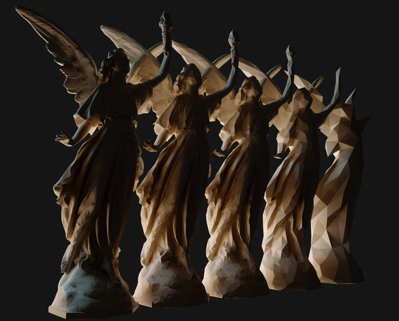
Triangle-Collapse
Edge-Collapse
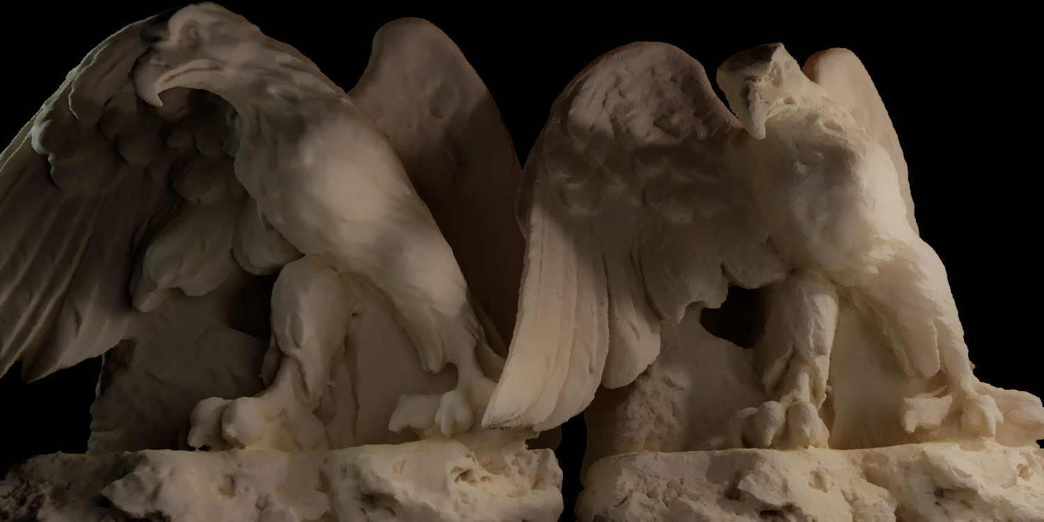
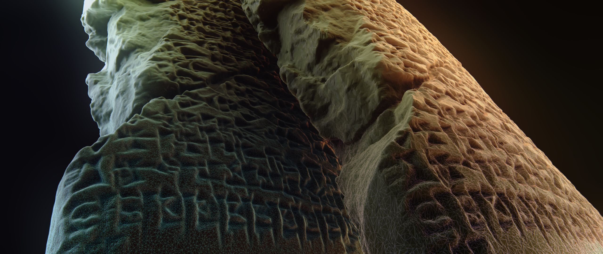
Lastly, this is one of the cases where Triangle-Collapse (apart from the cut-off podium) produces a much nicer looking output - especially when focusing on the wings and hair of the statue. It somehow is able to achieve a somewhat painterly look on a lot of models.
Performance
As already discussed in the Edge-Collapse entry, Triangle-Collapse is quite a lot faster in its current implementation than Edge-Collapse. For a more direct head-to-head comparison, let's take a look at performance metrics from the bird model shown in the Vertex-Elimination post. Please note, that Vertex-Elimination isn't even reaching anything close to 1/8 the triangle count, as it pollutes its own geometry with too many unfavourable polygons during the decimation process.
Target Tris
Step
Edge-Collapse
Triangle-Collapse
Vertex-Elimination
Initial Error Calc
0.08962 s
0.09059 s
0.09093 s
Error Sorting
0.09088 s
0.05267 s
0.02669 s
1/8
Decimation
4.75858 s
2.21628 s
0.60876 s
1/8
Out Verts
39,555
39,651
166,400
1/8
Out Tris
79,121
79,120
332,812
1/64
Decimation
5.24914 s
2.39596 s
1/64
Out Verts
4,942
5,095
1/64
Out Tris
9,889
9,887
1/256
Decimation
5.24396 s
2.43889 s
1/256
Out Verts
1,234
1,409
1/256
Out Tris
2,471
2,472
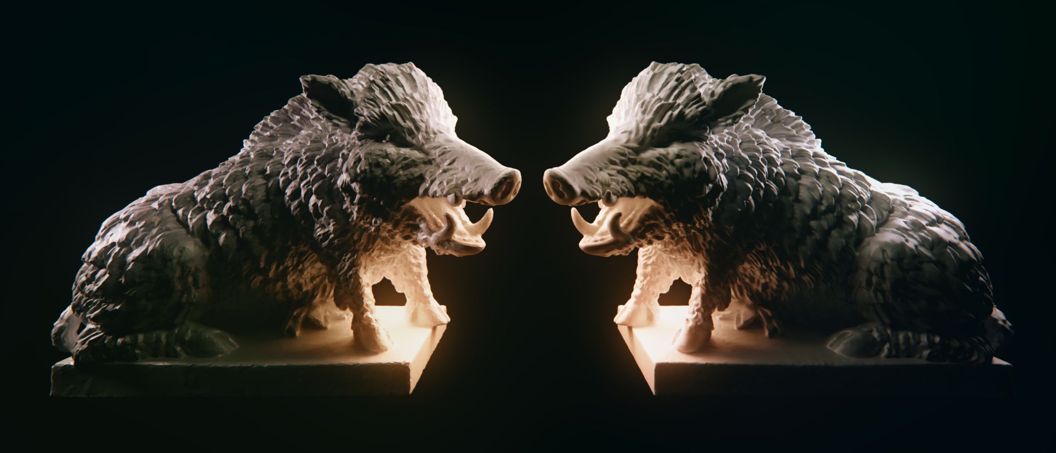
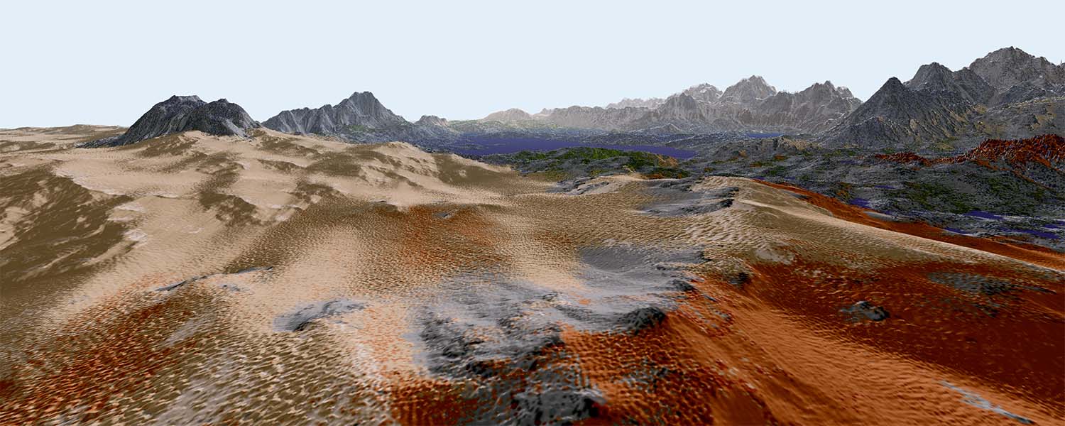
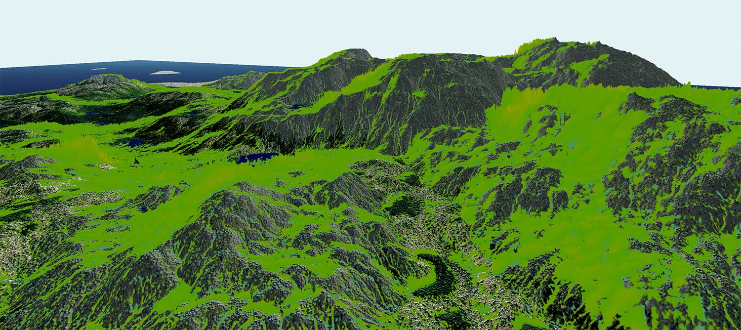
[Model of the Cover & second Image: Eber by noe-3d.at is licensed under Creative Commons Attribution-NonCommercial]
Mesh Decimation by Edge Collapse
Triangle-Collapse may be a terrific Mesh Decimation methodology for some scenarios, but for our specific requirements (Terrain LODs with certain immutable vertices at the edge) it isn't optimal as its caveats lie exactly in the areas that hurt the most. So, let's take our "Collapse"-Strategy one step back and - rather than collapsing entire triangles into a single vertex, merely collapse a single edge at a time.
Given the similarity to Triangle-Collapse, the implementation follows along the same lines: Pick an edge, update all triangles that touched the removed vertex to point to the remaining vertex instead and optionally update the remaining vertex position to a new position. We can choose to either collapse onto the center position of the edge, or pick the position of the vertex we consider to be more relevant (in our case the latter strategy is only used if one of the vertices is immutable). If a triangle contains both of the vertices, it can be removed entirely.
Performance
Edge-Collapse is unfortunately yet again a bit slower than Triangle-Collapse and Vertex-Elimination. To collapse the upper body of a high-resolution antique statue scan to 1/256 the vertex count we get the following metrics:
      Error Calculation: 2,370,474 edges / 790,872 verts in 9.19001 s (257,940 edges /s).

      Edge Reference Sorting: 0.02447 s (32,316,578 /s).

      Error Sorting:  0.21137 s (11,214,596 /s).

      Triangle Collapse: Removed 787,729 verts / 1573,439 tris in 18.53234 s (42,505 verts /s).


      Decimated: 790,872 verts, 1,579,609 tris to 3,143 verts, 6,170 tris.
This is unfortunately quite a lot slower for large models, but for our use case of decimating relatively small and low-complexity terrain geometry-fragments, this should still be acceptable.
Complications
Edge-Collapse isn't really more flexible, but more robust than Triangle-Collapse. Like Triangle-Collapse the strategy necessarily introduces averaged vertex positions into the mesh, but this didn't really cause any trouble with vertex-order or massive differences in any relevant scenarios yet. Sure, it's much slower - especially than the blazingly fast Vertex-Elimination, but it's robust and doesn't catch on fire if the source geometry isn't exactly to the specific tastes of the algorithm.
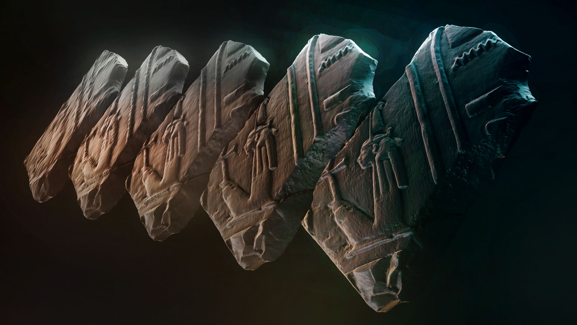
[Model of the Cover Image: Relief Depiction of Ma'at by IPCH Digitization Lab is licensed under Creative Commons Attribution]
Mesh Decimation by Triangle Collapse
As our Vertex-Elimination Decimation had too many caveats to be used as a general purpose decimation algorithm - and even ran into problems with our target of terrain decimation - we'll have to come up with a different solution. So, let's try to address the largest problems we ran into: Dependency on "nice" geometry, that we'd end up ruining eventually anyways & needing to do extra steps to fix vertex-ordering in triangles, if requested.
So how about if we don't start with vertices or lines - which may be part of complex polygons, but rather with triangles: Simply picking a triangle and collapsing it onto its barycenter should allow us to decimate even the most complex of meshes - with the downside, that with every collapse operation, we necessarily introduce a certain amount of inaccuracy, which may carry over into future collapses.
We can simply treat all of a triangle's vertices as references to the same remaining (now position-adjusted) result-vertex and ensure that all of their distinct neighbors reference this replacement vertex instead. If a neighbor triangle shares more than one vertex with our current triangle it can also be removed. We would assume triangle vertex order to stay consistent, as we're simply collapsing three vertices into one and don't really create any new vertices, but as no vertex position is "safe" from our decimation, it may occur, that triangles just happen to be collapsed into new positions that result in a flip of a triangle's vertex-order direction.
Our goal of restricting which vertices remain in place is slightly more difficult here, as we need to either not collapse any triangles that feature vertices that may not be moved or - if only one vertex may not be moved - collapse onto that vertex. In practice both of those strategies aren't flawless, especially since our mesh-generation scenario has to deal with a ton of open edges that may not be moved and need to line up exactly with another mesh's vertices - and the better of the two strategies happens to be the "not touching triangles with immutable vertices" one, which ends up severely limiting the level of decimation possible from a given input set of partially locked vertices.
Error Calculation
The error metric to prioritize triangles that collapse with the least amount of assumed visual difference can be fairly straightforward: Simply summing up the area of the 3d pyramid between the collapsed and non-collapsed vertex positions for each of the affected triangles (except the collapsed one) suffices.
Performance
Triangle-Collapse is unfortunately quite a lot slower than Vertex-Elimination, but still pretty fast. To collapse the upper body of a high-resolution antique statue scan to 1/256 the vertex count we get the following metrics:
      Error Calculation: 1,579,609 tris / 790,872 verts in 0.58253 s (2,711,622 tris /s).

      Error Sorting: 0.13659 s (11,564,442 /s).

      Triangle Collapse: Removed 787,256 verts / 1,573,441 tris in 7.59792 s (103,614 verts /s).


      Decimated: 790,872 verts, 1,579,609 tris to 3,616 verts, 6,168 tris.
The performance of Triangle-Collapse also benefits from the same chunked list data-structure, as implemented for Vertex-Elimination. For a more direct comparison, here's the metrics from running a light 1/8 decimation on the same model as in the Vertex-Elimination entry.
      Error Calculation: 632,974 tris / 316,481 verts in 0.23238 s (2,723,874.8 tris /s).

      Error Sorting: 0.05267 s (12,018,053 /s).

      Triangle Collapse: Removed 276,830 verts / 553,854 tris in 2.21628 s (124,907.4 verts /s).


      Decimated: 316,481 verts, 632,974 tris tris to 39,651 verts, 79,120 tris.
Complications
As already discussed, although much more flexible than Vertex-Elimination, Triangle-Collapse isn't without it's flaws. However, these are mostly limited to triangle vertex-ordering and necessarily introducing new vertex positions with every triangle collapse, so all-in-all it may be very much suitable for some use-cases. Triangle-Collapse can produce almost painterly features and is sometimes able to preserve sharp details much longer than other competing strategies, but unfortunately it wasn't a perfect match for ours.
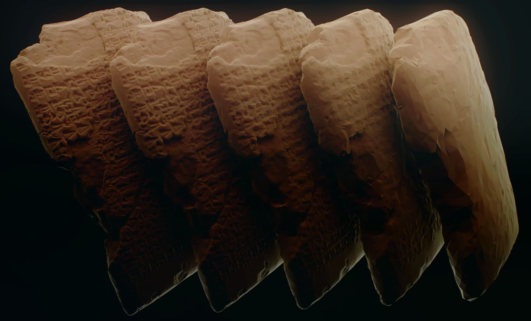
[Model in the Image below: Abecedary tablet by IPCH Digitization Lab is licensed under Creative Commons Attribution-NonCommercial]
Mesh Decimation by Vertex Elimination
Since Border-Alternating Terrain LODs require full control over which triangles are decimated, a custom mesh decimation algorithm is needed - and even if not, it'd be very convenient to have a fast, reliable & flexible way of decimation at our finger tips.
So decimating a mesh by eliminating the least-relevant vertices seemed like a novel & fast solution to the problem. But first, how do we want to eliminate those least-relevant vertices?
Let's assume, we have this geometry-fragment, and we've determined, that the tip of this shape is the vertex we'd like to eliminate. In order to remove said vertex from our object, we have to ensure, that all neighboring vertices that previously connected to the tip do now connect to one another. So, by observing the other vertices in all triangles connected with our chosen vertex, we can construct the polygon(s) of the resulting area. After sorting neighboring triangles into coherent polygons by finding common (= overlapping) vertices (which can be a bit tricky with "open" meshes or at the rims of mesh fragments, as there may not be any further overlapping vertices after a certain point, but still some triangles left to process), the polygon(s) can simply be triangulated and the chosen vertex has been eliminated.
As simple as this may seem, it sadly isn't that easy to implement in practice: Polygon triangulation in 3D isn't really a thing if the vertices don't all lie on a flat plane and even 2D polygon triangulation isn't trivial at all. As we're merely evaluating the suitability of this approach, we'll simply ignore those cases for now, and disallow any vertices from being eliminated if this would result in such a horrible case.
Regarding our goal of being able to leave singular vertices untouched, to line up with higher-fidelity LODs, this can be achieved very easily here, as the decimation procedure happens per-vertex anyways.
Error Calculation
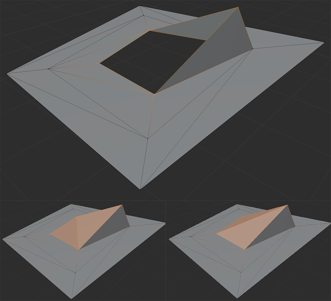
In order to prioritize vertices that result in minimal change to the mesh, we need to define an error function. Fortunately, this is rather easy: The error of removing the vertex at the tip can be formulated as the area between the re-triangulated base and the tip (= sum of the areas of the tetrahedron between the generated triangle and tip). As there's no singular valid triangulation of a polygon, this calculation unfortunately has to be repeated for all vertices and can't be blindly carried over to neighbors, as they may end up with a different triangulation, that would result in a different error value. To demonstrate, that not only one valid triangulation exists, let's consider the case of the following opening and its two different triangulations:
Performance
This approach is actually blazingly fast, even when forced to re-triangulate the resulting areas from the perspective of each vertex. To decimate the Statue pictured at the top of this entry (left) to the point where all vertex eliminations would result in horrific polygons (right), this is what we end up with:
      Error Calculation (incl. triangulation of base): 632,974 tris in 0.06161 s (3,449,320 non-skipped /s).

      Error Sorting: 0.02669 s (11,859,484 /s).

      Elimination & Re-Triangulation for 150,081 verts: 0.60876 s (246,536 /s).


      Decimated 316,481 verts, 632,974 tris to 166,400 verts, 332,812 tris. (removed 15,0081 verts, 300,162 tris)
This required an incredibly fast chunked list data-structure to be written, which allows for blazingly fast random removals & inserts (removing old error values in a sorted list, inserting new error values at the correct position) and a bunch of other little tricks.
Complications
What should now be somewhat apparent from the Performance Output above is, that many of the vertices needed to be skipped, as it would've been too complex to triangulate the resulting geometry. This usually isn't as terrible with smaller models, but heavily impacts the flexibility of this algorithm. What can be somewhat worked around, but isn't particularly pleasing about this approach is, that triangle vertex-ordering (which is sometimes used to determine normal directions and allows for front- or backface culling) isn't automatically preserved and needs to be fixed during the decimation process, if this behavior is relevant.
[Model of the Cover Image: Grabfigur by noe-3d.at is licensed under Creative Commons Attribution-NonCommercial] [Model in the Image below: Abecedary tablet by IPCH Digitization Lab is licensed under Creative Commons Attribution-NonCommercial]
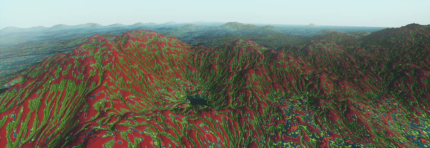
Border-Alternating Terrain LODs
With connected geometry - like terrain geometry - simply dissecting the model into tiles and providing various LODs for each tile (with larger tile sizes for lower quality LODs) unfortunately leads to problems whenever different LOD layers meet, as with a naive approach LOD levels would disagree at their borders about the level of fidelity. Forcing higher quality rims onto lower quality levels leads to an escalation, where even the lowest quality LODs would need to provide the highest quality borders, even though they would never actually border any of the highest quality levels, but as every lower level needs to be able to connect to a higher and lower quality level seamlessly, this forces highest quality borders onto all layers, which will increase the geometric detail of the lowest-quality LODs so much, that it entirely defeats the purpose of having LOD levels in the first place, as all of the detail is spent on irrelevant high-fidelity borders.
In order to resolve this, LOD levels can't share borders across all layers. This makes streaming LODs and generating LODs a lot more complex, but completely eliminates the issue at hand: Let's assume we have this lowest-quality LOD0 of our terrain.
If we want to load a segment of LOD0, we need to split it into its four children, as otherwise we'd end up rendering some segments twice: Once with LOD0 and more with LOD1.
Now, to address the issue discussed above: We need to choose a different boundary, at which higher-resolution LODs line up with LOD1. So, let's lock the vertices on the dark-turquoise lines to match the fidelity of LOD2.
Let's assume the worst case: We're interested in more detail in the selected tile of LOD2. Simply loading in this tile, we would disagree with the neighboring tiles of LOD1 on the level-of-fidelity at the two borders highlighted in white.
To address this, loading the tile highlighted in white forces the turquoise tiles to be loaded at the same LOD, as they share the same dark-turquoise square.
In order to again address the issue of sharing boundaries between LOD levels, we force the vertices on the dark-green lines to match the vertices at LOD3.
Let's again assume one of the more interesting cases, and let's say we want to load a higher quality LOD at the tile highlighted in green. Similar as before, this leads to a disagreement on the level of fidelity on the borders highlighed in white.
As discussed before, loading in the tile highlighted in white forces the tiles in green to be loaded as well. Actually any of these 4 tiles being loaded would force the remaining 3 tiles to be loaded in as well.
As two of the parent nodes of those nodes haven't been loaded in already, this also forces those parent nodes to be loaded in at a higher LOD as well, namely LOD2.
Implementing this intra-tile dependency isn't actually as tricky as it may seem, as it's always very straightforward to determine, which of the neighboring tiles need to be loaded in as well. A simple look-up-table suffices to store the vectors to the required neighboring ("sibling") tiles from the perspective of each child-index of a parent tile:
      static const vec2i8 siblings_from_child_idx[4][3]{

        {{-1, -1}, {0, -1}, {-1, 0}}, // top left

        {{0, -1}, {1, -1}, {1, 0}}, // top right

        {{-1, 0}, {-1, 1}, {0, 1}}, // bottom left

        {{1, 0}, {0, 1}, {1, 1}} // bottom right

      };
Now one can simply recursively iterate over tiles by starting at the root, splitting every tile that is sufficiently close and loading in all sibling tiles that need to be loaded alongside a given child.
Handling Procedural Geometry & Mesh Fragments
As we always need to know the vertices higher-resolution LOD layers in advance, it's highly recommended to generate such LODs with a bottom-up approach, as otherwise it's much more cumbersome to force our current LOD's vertices to match up with higher-resolution ones we haven't even seen yet. When doing so for partially loaded Meshes (especially common when procedurally generating or manipulating the underlying geometry), generating higher LOD layers with matching outer vertices (yes, not the inner vertices, that match up with higher LODs, but ones that need to match up with neighboring tiles of the same LOD level) can be tricky to handle. This is because neighboring LODs will be decimated separately, but we need to ensure that both we and them pick the same vertex positions on the rims of our tiles, as we'd end up with gaps between triangles otherwise. An easy strategy to handle this, is to manually Edge-Collapse every second vertex on the rim onto its neighbor, then mark the remaining rim vertices as immutable, before the entire tile is decimated to the desired level. This doesn't necessarily result in the most pleasing geometry, but it ensures consistency between the tiles and prevents any gaps from forming.
Single Bounce Voxel Traced Global Illumination
Now, that we've voxelized our shaded scene, the main deferred pass can be followed up by an additively blended global illumination pass. In this pass we use the same g-buffers as inputs as in the regular deferred shading pass, but instead of looking up lights and shading based on surface color and normal, we take the world-position as a starting point, reflect the camera-to-world-space-vector at the surface normal, move slightly (with a small random offset) into the derived direction (until we're no longer in the vicinity of neighboring voxels), add some random rotation to the direction vector (based on material roughness) and trace through the voxelized geometry until we either run out of steps (in this case, we assume, that we've hit the skybox and sample from it), or we've hit a shaded or unshaded populated voxel, in which case we derive the color from said voxel.
Even just sampling with one ray per pixel results in reasonably smooth results when viewed at sufficiently high framerates. This will eventually be smoothed out by TAA, so screenshots won't end up looking horribly noisy in the final version.
Effective Voxel Tracing
Given a voxel position pos (i.e. [1, 4, 7] in the voxel field [0, 0, 0] ~ [10, 10, 10]) and direction dir, with the sampled voxel being cpos = pos + t * dir, we can immediately transition to the next voxel by using the following basic formula:
Generating Randomly Rotated Vectors For Rough Surfaces
Randomly rotating arbitrary vectors can be somewhat cumbersome, we use the following approach:
Take the unit up-vector ([0, 0, -1] in our case)
Randomly rotate it in x and y direction (or whatever two directions aren't up in your preferred coordinate system)
Generate a mapping matrix, that rotates the unit up-vector onto our original vector using the previously discussed RotateAlignVectors function.
Transform the rotated up-vector with the mapping matrix
As this doesn't actually rotate arbitrary vectors but merely aligns the rotated vector with the up-vector, this approach doesn't suffer from the same issues as more straightforward implementations.
Hardware Voxelization
To be able to cheaply trace rays through the rendered scene, all static geometry is hardware voxelized through a clever combination of multisample anti-aliasing (MSAA) and a geometry shader that maximizes rasterized surface area.
As the color-resolution of the voxelized scene doesn't need to be particularly high or temporally stable, voxel colors are dithered and logarithmically encoded with only 8-bits per voxel (3 bits red, 3 bits green, 2 bits blue with 0 = no voxel).
Performant shading is provided through a world-space-clustering of the voxelized area, which works very similarly to the view-space clustering discussed previously, but instead of splitting the view-frustum into smaller pieces, the entire world-space in voxelizer range is split into regions, approximated by bounding spheres (if the voxelized area doesn't rotate, the bounding sphere calculation only needs to happen once, as all subsequent transforms are merely translations of the pre-existing clusters), then the bounding spheres are intersected with the light frustums in a cpu-side lighting pre-pass and stored in a separate lookup table.
Clustered Deferred Lighting
To significantly reduce the number of required shadow map lookups in a fragment shader, the view frustum can be subdivided into many small frustums in a pre-process (which we approximate by their bounding sphere). We can now check for the intersection of the light-view-frustum and view-frustum-segment-bounding-sphere and reference the relevant light indices of a given segment in a small lookup table.
Retrieving the corresponding cluster index in the fragment shader is very straightforward, as the only information required to resolve the fragment to a cluster is the screenspace texture coordinate and linearized depth ratio between the near and far plane. All of these inputs are already commonplace in deferred shading setups.
Additionally, such a lookup can easily be utilized to implement a basic volumetric lighting shader.
Procedurally generated PBR textures
To fill our procedurally generated worlds with unique looking environments, we render the corresponding colors for a given region directly into the texture atlas.
As material indexes are directly passed to the shader, alongside the world-position of the corresponding terrain, we can select the correct type of texture and procedurally generate the values to the atlas. This results in a lot of variety, even if the same material is used:
Snowy Rocks
Ice
Blending is done on by simply applying a noise function to the barycentric coordinates that are used to fetch the per-vertex material index in the fragment shader from a texture. Sadly it's currently not possible to use different noise patterns for different kinds of material combinations, but the current noise pattern results in very pleasing material transitions already (see video in the header)
This way we can create a wide variety of procedural textures and selectively apply them to the underlying terrain. These are all of the material types we currently offer:
Improving and Optimizing the Texture Atlas
The original implementation was already capable of processing hundreds of thousands of triangles per second, but the utilization of the texture area wasn't particularly good, as the coverage quadtree initially preferred placing triangle clusters at high-layer node positions. This left arbitrarily sized holes in the quadtree that are neither particularly easy to find, when looking for available space for future clusters nor necessarily good spots to place clusters into, as the total available area is quickly fragmented by the first couple of clusters.
We'd much prefer clusters to be placed closer to existing clusters, so we'll modify the atlas slightly: After the final dimensions have been found, we allow the quadtree to attempt to move the current bounds to the top left by one node per layer if possible. This achieves much better atlas coverage - still not optimal, but improved to the point that models with double the unit-size can consistently fit into the atlas now. Apart from the coverage benefits, for some models this ends up positively impacting the runtime performance as well, as it's much faster to find empty spots with the improved coverage.
After a bunch of smaller optimization (mostly bloom-filters to avoid costlier randomish-memory-access-dependent-conditionals) we're somewhere between handling 500k - 1M Triangles per Second on a single thread.
Stanford Dragon Texture Coordinates & Model Render
To actually get a decent performance benchmark of the texture atlas, I fed it the entire stanford dragon model (871k Triangles), as well as a bunch of other large standard models (like a simplified version of Stanford Lucy).
      2.01443 s (432,422 triangles per second) without moving cluster bounds to the top-left

      0.87905 s (990,936 triangles per second) with moving cluster bounds to the top-left
Although, with the simplified Stanford Lucy model however (28k Triangles), the old method appears still to be faster - probably because of the larger variance in terms of triangle area:
      0.02538 s (1,105,358 triangles per second)  without moving cluster bounds to the top-left

      0.05534 s (506,846.8 triangles per second)  with moving cluster bounds to the top-left
Fast Texture Atlas for Procedural Geometry
Since world chunks are going to be represented with consistent, but procedural geometry, we need an efficient way of generating texture information for chunks to make manual changes and unique-looking locations possible. To sample and store the corresponding texture, we need an efficient way of generating texture coordinates for our procedural geometry.
As many existing texture atlas implementations aren't particularly fast or assume that the geometry already comes with UV partitioning and texture coordinates that only need to be assembled into one big atlas, I chose to implement a new texture atlas system for the engine.
The foundation of the texture atlas is a coverage-quadtree where nodes are either empty, partially-covered or full. Nodes are stored in a large buffer as there's no need to stream information on demand. The last layer is merely represented as a large bitmap, rather than the actual nodes containing information about the pixel contents. Utilizing this coverage-quadtree it's fairly straightforward to check if a certain amount of space is currently available in the atlas.
The atlas procedure consists of two steps:
Setup
Add all triangles with 3d position and vertex indexes to the atlas. The atlas calculates the side lengths and angles of the triangle and takes note of existing triangles that share an edge with the current one.
Texture Coordinate Generation
After all triangles have been added, they are first sorted by area. Then chunks of triangles are attempted to be added to the atlas branching out from the initial large triangle's edges.
There's some special cases that have to be handled here, like when all three vertexes of a triangle are already present in the atlas and connecting them into a new triangle would result in a reasonable approximation of sizes and angles in respect to the original 3d geometry. Likewise, in order to ensure that the resulting areas don't get out of hand with curved geometry, as angles are used to construct the 2d triangles in the texture atlas and the resulting area may slowly creep up or down in size compared to their 3d counterparts, mismatching triangles are rejected from the current batch and will either be added separately or as part of another triangle-cluster.
Whenever no more connecting triangles would fit into the area available in the texture atlas, triangle bounds are marked as covered and we move on to the next possible collection of triangles - starting with the next largest triangle that hasn't been placed yet.
Obviously this doesn't result in optimal utililzation of the texture atlas, especially as the bounding rectangle of a triangle is a terrible estimate of it's actual coverage, but this comes with a large performance benefit, as no triangle rasterization is required and the texture generation part can be offloaded to the GPU.
Pixels, Shell Texturing & Grass Height
Achieving tripple-A quality graphics isn't entirely feasible with just the limited time of one person, so choosing a distinct, pleasant, and lower-fidelity art-style is very important. To force myself to think more about the broad picture than the low-level details, I halved the display resolution, using my trusty old aliasing-pixelartify algorithm for a neat pixely look.
Now to the fun part: Moss. Well, shell texturing.
To supplement the grass and enable moss growth on rocks and other similar surfaces, we create a vegetation-height map that is a half-terrain-resolution approximation of the height of grass - or only moss, if the values are too low to allow grass to grow. We can now color the grass depending on the length to achieve some more visual interest.
For moss, we create two LODs of instanced heightmap textures with varying height attribute. We create a moss height, normal direction & color change texture that is statically used for all moss and sample the depth from this texture in the fragment shader to conditionally discard (I don't want to, but alpha blending would be a lot worse) fragments.
Giving the height channel some bumps here and there and sampling a different color depending on the moss height leaves us with a nice fluffy mossy texture that nicely complements the grass.
Grass Rendering & Chunk View Culling
Flat untextured terrain however isn't particularly pleasing to look at, so - after implementing a chunk view culling system and reducing the draw-calls for terrain rendering to one draw-call per chunk type and refactoring the renderer a bit, let's have a look at grass rendering.
I'm not the biggest fan of alpha textured grass rendering as the constant overdraw fragment discarding sounds very unpleasant to me. As modern GPUs are capable of rendering a lot of instanced geometry very quickly and having individual segmented blades of grass allows for nice curving grass in the wind, we'll use that approach. Depending on how close the chunk containing the grass is to the camera, we'll use a different LOD on the grass segmentation as even reasonably close chunks can visually represent blades of grass with just a single triangle without a perceptual loss in quality.
This doesn't cover chunks yet, that are further off in the distance, but depending on how well we can tune the shaders later on, we might be able to either render billboards with large amounts of grass, or even fake the existence of grass entirely with a decent grass-landscape texture.
Terrain Chunk Streaming & Atmospheric Effects
In order to traverse such a large scale terrain, LOD & streaming need to be considered immediately. Chunks of different sizes are streamed into fixed-size textures and are dynamically loaded when needed.
Whenever a large chunks would contain a chunk with vertexes that are closer than a set distance from the camera, the chunk is split and the contained chunks of higher fidelity are streamed in.
To reduce the pop-in artifacts usually seen in even tripple-A productions, we use local maxima - rather than average terrain height - to construct LODs.
Obviously this leaves visible gaps in the landscape wherever multiple chunk-types meet, but we'll deal with specific meshes to solve this problem at a later date.
A low LOD texture atlas
Atmospheric Effects
The sun position is now 'rotated' into the coordinate space mapped around the 'flat' planet and camera position using a vector alignment matrix:
The way the sun passes through the atmosphere is approximated with an iterative shader that draws an equirectangular view and approximates rayleigh and mie scattering with a fixed number of samples. The scale of the planetary system and atmosphere have been adjusted to achieve earth-like atmospheric conditions.
Micro-Biome Extraction
After the terrain has been generated and eroded, regions need to be classified into biomes based on the physical properties of their surroundings. To calculate these biomes like various grass types wherever the top soil is grass a noise map can be sampled. However this isn't entirely accurate as especially regional & global elevation changes and water proximity can influence biome parameters significantly.
Therefore we compute a signed distance field of water and one that maps terrain height, blur the height map over a large area and then compute the local difference to an areas neighbors. This leaves us with the water map and the map shown above for local terrain elevation changes.
Using these two maps and a noise buffer, we can derive micro-biome features like mossy stones near water or in crests, small puddles can be turned to mud, large elevation change inhibit the growth of trees or tall grass, ...
Wind Erosion
With our newly developed surface wind simulation, we can now erode the surface terrain. Terrain that's close to the wind height will be eroded more than terrain that's further from it and wind speeds influence how far particles are dragged when eroded. The various terrain layers have different properties of how easily they can be erroded by wind & water.
As the eroded particles are dragged through the wind, the terrain is iteratively checked for matching height as the particles slowly descend based on their weight.
Similarly to the wind simulation, eroded particles are added onto a separate buffer and are applied to the new terrain after all cells have completed their erosion procedure.
Simulating Wind
In order to arrive at realistic wind conditions to drive wind erosion, both atmospheric and surface conditions must be simulated. The atmospheric wind simply boils down to
Generally air is dragged in the opposite direction of the planetary rotation through the coriolis force.
The air in each atmospheric cell warms up based on solar energy reaching the surface (and slowly cools to the temperature of outer space when there's no incoming solar energy)
Based on the temperature and the air density at any position, calculate the pressure
Move air-mass (density) velocity around to attempt to equally distribute air pressure
The last step can be applied iteratively to support fine-grained air movements. Whilst iterating the exiting wind buffer, resulting wind is accumulated in a separate buffer to be applied after all cells have been processed.
One trick that specifically helped simulating sub-cell movements over multiple iterations - by slightly breaking the laws of physics - was to multiply the wind speeds in cells that don't have enough wind speed to make any pressure move from one cell to the next. This eventually tips the scales and makes the wind in those low pressure cells travel small distances over large amounts of time consistently.
Atmospheric Air Density and Wind Speed Vectors
Surface Wind
Surface wind derives its temperature from the reflectivity and temperature emission of the underlying material. Surface Wind can be imaginged as a sheet of cloth that's being dragged over the terrain surface. Wind Speeds slow down (in my implementation even reverse slightly) when moving against higher terrain. This may result in the wind height being raised at a given position, or the wind preferring another direction over the current brute-force approach.
Falling winds to the contrary even enjoy a slight speedup to their wind speeds. This results in pressure zones being separated by mountain ranges whilst wind bursts through the cracks in order to equalise the pressure on both sides.
Surface winds are slightly dragged along with the general atmospheric wind.
Surface Air Density and Wind Speed Vectors
Orbital Dynamics
In order to have semi-accurate climatic conditions producing terrain with only one hot and one cold zone, an somewhat excentric elliptic orbital path with fine tuned rotational velocity and direction is required. Solving orbital dynamics formulas - even with a fixed star that isn't affected by the satellites mass - proved quite difficult however.
In Polar Coordinates, the orbital distance from the origin at angle theta with orbital parameters a and b can be expressed like this:
radius(theta) := (a * (1 - b * b)) / (1 + b * cos(theta))
This alone doesn't help much however, as the velocity at each position can easily be calculated, but woulnd't translate to a closed form solution and I didn't want to resort to step-wise simulation that'd be hard to rely on or accurately predict with different time steps. So, I was able to construct a function angle(time) to derive the radius by pluggin the result into the radius function:
In order to arrive at a combined mass that actually produces a period of 2 * pi, we have to calculate the mass from orbital parameter a:
combinedMass(a) := (2 * a * pi / 2) / (pi * pi)
As the combined mass of the two orbital bodies doesn't change with the system, it can be calculated on initialization when setting the other orbital parameters.
Planets, Average Solar Energy on the Surface, Current Solar Energy
Hydrolic Erosion
The layered terrain can be eroded using simulated water-droplets that carry material based amounts of sediment around. Finding the path to the deepest reachable point (or until all water has evaporated) for each block of terrain is vastly faster than simulating only one step at a time, but produces much rougher terrain than stepwise erosion. Stepwise erosion smoothes out the terrain and forms large water streams that then decend down to the valleys, where the small crests created from the first few water droplets in the decent-per-droplet approach won't widen and will preferrably be used by later droplets that run down similar paths, not resulting in broadening of common water paths.
Layered Terrain Before / After Water Erosion
Layer Based Terrain
Terrain is built in layers, the bottom layer is non-erodable bedrock. Depending on a signed-distance field, a noise layer and two cubic slopes a certain height of terrain of a given layer will be added on top of the existing terrain. The signed distance field chooses the min and max value from the two cubic slopes (basically a min- and max height) and the noise value (between 0 and 1) is used to smoothly interpolate between those two values. The generated terrain is rough at first, but erosion will massively improve and shape those layers later.
const float_t min = a_min * x * x * x + b_min * x * x + c_min * x + d_min;
const float_t max = a_max * x * x * x + b_max * x * x + c_max * x + d_max;
const float_t height = lerp(min, max, noiseValue);